---
title: Auto Operating Costs Calculation
subtitle: Estimating Auto Operating Costs for Travel Demand Model
author:
- name: Pukar Bhandari
email: pukar.bhandari@wfrc.utah.gov
affiliation:
- name: Wasatch Front Regional Council
url: "https://wfrc.utah.gov/"
date: "2025-09-17"
---
This document updates the `0 - Auto Operating Cost - 2022-01-11.qmd` to the new base year `2023`.
## Instruction
This analysis calculates auto operating costs for different vehicle classes using a base year of 2023. Operating costs represent the variable expenses incurred per mile of vehicle travel, primarily fuel and maintenance. These costs are critical inputs for travel demand models, which use them to predict how people make transportation choices based on the relative costs of driving.
The methodology combines data from multiple federal agencies. The Bureau of Transportation Statistics (BTS) provides historical data on fuel prices, vehicle expenditures, fleet characteristics, and average costs of vehicle ownership. The Energy Information Administration (EIA) supplies detailed regional fuel price data specific to the Rocky Mountain area, which includes Utah and neighboring states. The Bureau of Labor Statistics (BLS) provides the Consumer Price Index, allowing us to adjust historical costs for inflation. The American Automobile Association (AAA) publishes annual driving cost surveys that break down expenses into variable and fixed components. Finally, the Oak Ridge National Laboratory maintains the Transportation Energy Data Book with detailed fuel economy statistics by vehicle size class.
By synthesizing these diverse data sources, we can identify long-term trends, compare actual costs against historical patterns, and produce defensible estimates for current-year operating costs across four vehicle classes: automobiles (passenger cars), light-duty trucks (pickups and SUVs), medium-duty trucks (single-unit delivery trucks), and heavy-duty trucks (tractor-trailers).
## Environment Setup
### Load Libraries
``` python
!conda install numpy pandas geopandas matplotlib seaborn scipy openpyxl python-dotenv tabula-py
```
```{python}
# For Analysis
import numpy as np
import pandas as pd

# For Visualization
import matplotlib.pyplot as plt
import matplotlib.dates as mdates
from matplotlib.ticker import FuncFormatter
import seaborn as sns
from scipy.interpolate import make_interp_spline
from scipy import stats

# misc
import datetime
import os
from pathlib import Path
import requests
import tabula
import re
```
### Set Base Year for Calculations
```{python}
BASE_YEAR = 2023
```
## Define Helper Functions
To maintain code reusability and follow DRY (Don't Repeat Yourself) principles, we define helper functions for common operations throughout the analysis.
### Fetch Excel Files from BLS or BTS
This utility function automates downloading data files from federal agencies. It checks if a file already exists locally before attempting to download, avoiding unnecessary network requests and respecting the agencies' servers. The function includes proper HTTP headers to ensure reliable downloads.
```{python}
def ensure_exists(path, url):
    """
    Download Excel file if it doesn't exist locally.

    Parameters:
    -----------
    path : str or Path
        Local file path to save the Excel file
    url : str
        URL to download the Excel file from
    """
    # Convert to Path object if string
    filepath = Path(path)

    # Download file if it doesn't exist
    if not filepath.exists():
        filepath.parent.mkdir(parents=True, exist_ok=True)

        headers = {
            'User-Agent': 'Mozilla/5.0 (Windows NT 10.0; Win64; x64) AppleWebKit/537.36'
        }

        response = requests.get(url, headers=headers)
        filepath.write_bytes(response.content)
```
## Read Raw Data
The data collection process is designed for reproducibility and transparency. Each dataset is automatically downloaded from its authoritative source and cached locally in the `data/` directory. The code checks whether files already exist before attempting downloads, which speeds up subsequent runs and reduces load on source servers.
For each dataset, the code specifies the exact file location, sheet name (for Excel files), header row, columns to read, and number of rows to process. This explicit specification ensures that anyone running this analysis will extract identical data. Comments in the code indicate which columns may need updating as new data becomes available in future years.
Some datasets require special handling. The Consumer Price Index data is fetched via the BLS API, which requires a free API key stored in a `.env` file. The AAA driving costs data is extracted from a PDF using the `pdfplumber` library, which parses table structures from the formatted document. Column names containing year information are cleaned and standardized using regular expressions to ensure consistent formatting.
### 3-11
Table 3-11 provides historical fuel prices to end-users from 1970 through the most recent year available. This dataset includes separate price series for gasoline, diesel, and other fuel types across all states. While we primarily rely on EIA data for detailed regional pricing, this BTS table provides context for long-term national trends.
Table 3-11: Sales Price of Transportation Fuel to End-Users \[Source: [Bureau of Transportation Statistics](https://www.bts.gov/content/sales-price-transportation-fuel-end-users-current-cents-gallon)\]
```{python}
#| eval: false
# Set file path and source URL
filepath_3_11 = Path("data/bts/table_03_11_032824.xlsx")
url_3_11 = "https://www.bts.gov/sites/bts.dot.gov/files/2024-03/table_03_11_032824.xlsx"

# Ensure the file exists, Download if not
ensure_exists(path=filepath_3_11, url=url_3_11)

# Read Excel file
df_3_11 = pd.read_excel(
  filepath_3_11,
  sheet_name="3-11",
  header=1,
  usecols="A:AK", # TODO: update cols later for new data
  nrows=10
)

# display the data
df_3_11
```
### 3-12
Table 3-12 tracks how gasoline prices have changed relative to other consumer goods and services. This relative price index reveals whether fuel costs are rising faster or slower than general inflation. When gasoline prices rise faster than overall inflation, transportation becomes relatively more expensive, potentially shifting travel behavior toward more efficient modes or shorter trips.
Table 3-12: Price Trends of Gasoline v. Other Consumer Goods and Services \[Source: [Bureau of Transportation Statistics](https://www.bts.gov/content/price-trends-gasoline-v-other-consumer-goods-and-services)\]
```{python}
#| eval: false
# Set file path and source URL
filepath_3_12 = Path("data/bts/table_03_12_032824_1.xlsx")
url_3_12 = "https://www.bts.gov/sites/bts.dot.gov/files/2024-03/table_03_12_032824_1.xlsx"

# Ensure the file exists, Download if not
ensure_exists(path=filepath_3_12, url=url_3_12)

# Read Excel file
df_3_12 = pd.read_excel(
  filepath_3_12,
  sheet_name="3-12",
  header=1,
  usecols="A:AM", # TODO: update cols later for new data
  nrows=15
)

# display the data
df_3_12
```
### 3-25
Table 3-25 shows average wages in transportation industries, which provides economic context for understanding how transportation costs relate to household incomes. While not directly used in operating cost calculations, this data helps validate that our cost estimates are reasonable relative to what workers in the transportation sector earn.
Table 3-25: Average Wage and Salary Accruals per Full-Time Equivalent Employee by Transportation Industry \[Source: [Bureau of Transportation Statistics](https://www.bts.gov/content/average-wage-and-salary-accruals-full-time-equivalent-employee-transportation-industry-naics)\]
```{python}
#| eval: false
# Set file path and source URL
filepath_3_25 = Path("data/bts/table_03_25_102122.xlsx")
url_3_25 = "https://www.bts.gov/sites/bts.dot.gov/files/2022-10/table_03_25_102122.xlsx"

# Ensure the file exists, Download if not
ensure_exists(path=filepath_3_25, url=url_3_25)

# Read Excel file
df_3_25 = pd.read_excel(
  filepath_3_25,
  sheet_name="3-25",
  header=1,
  usecols="A:Y", # TODO: update cols later for new data
  nrows=10
)

# display the data
df_3_25
```
### 4-12
Table 4-12 details fuel consumption and vehicle miles traveled for light-duty vehicles with long wheelbases—primarily SUVs, vans, and pickup trucks. This category represents a significant and growing share of the passenger vehicle fleet. The table reports both fuel consumed (in millions of gallons) and miles traveled (in billions), which together yield fuel economy in miles per gallon.
Table 4-12: Light Duty Vehicle, Long Wheel Base Fuel Consumption and Travel \[Source: [Bureau of Transportation Statistics](https://www.bts.gov/content/other-2-axle-4-tire-vehicle-fuel-consumption-and-travel-0)\]
```{python}
#| eval: false
# Set file path and source URL
filepath_4_12 = Path("data/bts/table_04_12M_032725.xlsx")
url_4_12 = "https://www.bts.gov/sites/bts.dot.gov/files/2025-03/table_04_12M_032725.xlsx"

# Ensure the file exists, Download if not
ensure_exists(path=filepath_4_12, url=url_4_12)

# Read Excel file
df_4_12 = pd.read_excel(
  filepath_4_12,
  sheet_name="4-12M",
  header=1,
  usecols="A:AM", # TODO: update cols later for new data
  nrows=6
)

# display the data
df_4_12
```
### Fuel Economy - CombinedVehType
Table 4-9 aggregates fuel consumption and travel across all motor vehicle types. This provides a fleet-wide perspective on average fuel economy and helps ensure that our vehicle-class-specific estimates align with national totals. The combined data includes passenger cars, light trucks, buses, and heavy trucks.
Table 4-9: Motor Vehicle Fuel Consumption and Travel \[Source: [Bureau of Transportation Statistics](https://www.bts.gov/content/motor-vehicle-fuel-consumption-and-travel)\]
```{python}
#| eval: false
# Set file path and source URL
filepath_4_9 = Path("data/bts/table_04_09_032825.xlsx")
url_4_9 = "https://www.bts.gov/sites/bts.dot.gov/files/2025-03/table_04_09_032825.xlsx"

# Ensure the file exists, Download if not
ensure_exists(path=filepath_4_9, url=url_4_9)

# Read Excel file
df_FE_CombinedVehType = pd.read_excel(
  filepath_4_9,
  sheet_name="4-9",
  header=1,
  usecols="A:AO", # TODO: update cols later for new data
  nrows=6
)

# display the data
df_FE_CombinedVehType
```
### Fuel Economy - LightDuty
Table 4-23 focuses specifically on light-duty vehicles (passenger cars and light trucks under 8,500 pounds). This is the most detailed fuel economy dataset for the vehicles that comprise the majority of personal travel. The table separates passenger cars from light trucks and tracks how fuel economy has improved over time due to Corporate Average Fuel Economy (CAFE) standards and technological improvements in engines, transmissions, and vehicle design.
Table 4-23: Average Fuel Efficiency of U.S. Light Duty Vehicles \[Source: [Bureau of Transportation Statistics](https://www.bts.gov/content/average-fuel-efficiency-us-light-duty-vehicles)\]
```{python}
# Set file path and source URL
filepath_4_23 = Path("data/bts/table_04_23_042425.xlsx")
url_4_23 = "https://www.bts.gov/sites/bts.dot.gov/files/2025-04/table_04_23_042425.xlsx"

# Ensure the file exists, Download if not
ensure_exists(path=filepath_4_23, url=url_4_23)

# Read Excel file
df_FE_LightDuty = pd.read_excel(
  filepath_4_23,
  sheet_name="4-23",
  header=1,
  usecols="A:AK", # TODO: update cols later for new data
  nrows=12
)

# display the data
df_FE_LightDuty
```
### Personal Expenditure
Table 3-15 shows total personal consumption expenditures across all categories: housing, healthcare, food, transportation, and others. Transportation typically represents 15-20% of household budgets. By tracking transportation's share over time, we can assess whether our operating cost estimates produce results consistent with observed household spending patterns. The column names are cleaned to extract just the year, removing formatting artifacts like "(R)" revision markers.
Table 3-15: Personal Expenditures by Category (Millions of current dollars) \[Source: [Bureau of Transportation Statistics](https://www.bts.gov/content/personal-expenditures-category-millions-current-dollars)\]
```{python}
#| eval: false
# Set file path and source URL
filepath_3_15 = Path("data/bts/table_03_15_022525.xlsx")
url_3_15 = "https://www.bts.gov/sites/bts.dot.gov/files/2025-02/table_03_15_022525.xlsx"

# Ensure the file exists, Download if not
ensure_exists(path=filepath_3_15, url=url_3_15)

# Read Excel file
df_PersonalExpenditure = pd.read_excel(
  filepath_3_15,
  sheet_name="3-15",
  header=1,
  usecols="A:AP", # TODO: update cols later for new data
  nrows=17
)

# Extract years from column names, handling formats like "(R) 2019"
df_PersonalExpenditure.columns = [
    str(int(match.group())) if (match := re.search(r'\b(19|20)\d{2}\b', str(col))) else col
    for col in df_PersonalExpenditure.columns
]

# display the data
df_PersonalExpenditure
```
### Personal Consumption
Table 3-16 breaks down transportation expenditures into subcategories: vehicle purchases, gasoline and oil, maintenance and repairs, insurance, and public transportation. This detailed breakdown allows us to isolate the specific cost components we're estimating and compare our calculations against actual household expenditure data reported in national accounts.
Table 3-16: Personal Consumption Expenditures on Transportation by Subcategory (Millions of current dollars) \[Source: [Bureau of Transportation Statistics](https://www.bts.gov/content/personal-consumption-expenditures-transportation-subcategory-millions-current-dollars)\]
```{python}
#| eval: false
# Set file path and source URL
filepath_3_16 = Path("data/bts/table_03_16_022525.xlsx")
url_3_16 = "https://www.bts.gov/sites/bts.dot.gov/files/2025-02/table_03_16_022525.xlsx"

# Ensure the file exists, Download if not
ensure_exists(path=filepath_3_16, url=url_3_16)

# Read Excel file
df_PersonalConsumption = pd.read_excel(
  filepath_3_16,
  sheet_name="3-16",
  header=1,
  usecols="A:AP", # TODO: update cols later for new data
  nrows=17
)

# display the data
df_PersonalConsumption
```
### Consumer Price Index
The Consumer Price Index (CPI-U) measures the average change in prices paid by urban consumers for a basket of goods and services. The BLS API provides monthly CPI values from 1913 to the present. We calculate annual averages and year-over-year percent changes to track inflation. The CPI serves multiple purposes in this analysis: adjusting historical costs to constant dollars, comparing how auto costs change relative to general inflation, and normalizing costs across different time periods. The API requires a free registration key, which should be stored in a `.env` file to keep it secure and separate from the code.
Data Source: Consumer Price Index for All Urban Consumers (CPI-U) \[Source: [Bureau of Labor Statistics](https://data.bls.gov/pdq/SurveyOutputServlet)\]
::: {.callout-tip}
Get your BLS Public API key from [here](https://data.bls.gov/registrationEngine/).
Create a `.env` file in the root directory and add your BLS API key:
```BLS_PUBLIC_API=your-key-here```
This enables fetching Consumer Price Index data from the BLS API.
:::
```{python}
from dotenv import load_dotenv
load_dotenv()
```
```{python}
# Ensure file exists
filepath_cpi = Path("data/bls/cpi_1913_present.xlsx")

if not filepath_cpi.exists():
    filepath_cpi.parent.mkdir(parents=True, exist_ok=True)

    api_url = "https://api.bls.gov/publicAPI/v2/timeseries/data/"
    current_year = pd.Timestamp.now().year
    all_data = []

    for start_year in range(1913, current_year + 1, 20):
        end_year = min(start_year + 19, current_year)
        payload = {
            "seriesid": ["CUUR0000SA0"],
            "startyear": str(start_year),
            "endyear": str(end_year),
            "catalog": False,
            "calculations": False,
            "annualaverage": False,
            "registrationkey": os.getenv('BLS_PUBLIC_API')
        }
        response = requests.post(api_url, json=payload, headers={"Content-Type": "application/json"})

        for item in response.json()['Results']['series'][0]['data']:
            if item['period'].startswith('M') and item['period'] != 'M13':
                all_data.append({
                    'year': int(item['year']),
                    'period': item['period'],
                    'value': float(item['value'])
                })

    df_pivot = pd.DataFrame(all_data).pivot(index='year', columns='period', values='value')
    df_pivot = df_pivot[[f'M{i:02d}' for i in range(1, 13)]].sort_index()

    with pd.ExcelWriter(filepath_cpi, engine='openpyxl') as writer:
        df_pivot.to_excel(writer, sheet_name='BLS Data Series')

# Read Excel file directly from URL
df_CPI = pd.read_excel(
  filepath_cpi, # File path
  sheet_name="BLS Data Series",
  usecols="A:M" # TODO: update cols later for new data
)

# Calculate annual average
df_CPI['annualaverage'] = df_CPI[[f'M{i:02d}' for i in range(1, 13)]].mean(axis=1)

# Calculate 12-month percent change for December
df_CPI['pct_change_Dec'] = df_CPI['M12'].pct_change(periods=1, fill_method=None) * 100

# Calculate 12-month percent change for annual average
df_CPI['pct_change_Avg'] = df_CPI['annualaverage'].pct_change(periods=1, fill_method=None) * 100

# display the data
df_CPI
```
### Retail Diesel Prices
The EIA publishes weekly retail diesel prices by region. Diesel fuel powers medium-duty and heavy-duty trucks, so accurate diesel pricing is essential for calculating operating costs for freight vehicles. The Rocky Mountain region pricing reflects conditions in Utah, Colorado, Wyoming, Montana, and Idaho. Diesel prices typically run 10-20% higher than gasoline due to higher refining costs and federal excise tax rates, though the spread varies with crude oil prices and refinery economics.
Retail Prices for Diesel (On-Highway) - All Types \[Source: [Energy Information Administration](http://www.eia.gov/dnav/pet/pet_pri_gnd_a_epd2d_pte_dpgal_w.htm)]
```{python}
# Set file path and source URL
filepath_retaildiesel = Path("data/eia/PET_PRI_GND_A_EPD2D_PTE_DPGAL_W.xls")
url_retaildiesel = "https://www.eia.gov/dnav/pet/xls/PET_PRI_GND_A_EPD2D_PTE_DPGAL_W.xls"

# Ensure the file exists, Download if not
ensure_exists(path=filepath_retaildiesel, url=url_retaildiesel)

# Read Excel file directly from URL
df_RetailDieselPrices = pd.read_excel(
  filepath_retaildiesel, # File path
  sheet_name="Data 2",
  header=2,
  usecols="A:J" # TODO: update cols later for new data
)

# display the data
df_RetailDieselPrices
```
### Retail Gas Prices
Similar to diesel prices, the EIA provides weekly retail gasoline prices for all grades (regular, midgrade, premium) by region. Most light-duty vehicles use regular gasoline, though some require premium. The "all grades" series provides a weighted average that reflects actual consumer purchasing patterns. Weekly data captures seasonal price fluctuations—prices typically rise in summer due to higher driving demand and the switch to more expensive summer-blend fuel formulations required for air quality.
Retail Prices for Gasoline, All Grades \[Source: [Energy Information Administration](https://www.eia.gov/dnav/pet/pet_pri_gnd_a_epm0_pte_dpgal_w.htm)]
```{python}
# Set file path and source URL
filepath_retailgas = Path("data/eia/PET_PRI_GND_A_EPM0_PTE_DPGAL_W.xls")
url_retailgas = "https://www.eia.gov/dnav/pet/xls/PET_PRI_GND_A_EPM0_PTE_DPGAL_W.xls"

# Ensure the file exists, Download if not
ensure_exists(path=filepath_retailgas, url=url_retailgas)

# Read Excel file directly from URL
df_RetailGasPrices = pd.read_excel(
  filepath_retailgas, # File path
  sheet_name="Data 2",
  header=2,
  usecols="A:J" # TODO: update cols later for new data
)

# display the data
df_RetailGasPrices
```
### Average Cost
Table 3-17 reports the average cost of owning and operating an automobile assuming 15,000 miles of annual driving. AAA compiles this data annually through surveys and manufacturer specifications. The costs are broken into variable expenses (fuel, maintenance, tires) that increase with miles driven, and fixed expenses (insurance, license/registration/taxes, depreciation, finance charges) that remain relatively constant regardless of mileage. This decomposition is critical because travel demand models respond primarily to variable costs—travelers notice the cost of each additional mile driven, but fixed costs are sunk regardless of how much they drive.
Table 3-17: Average Cost of Owning and Operating an Automobilea (Assuming 15,000 Vehicle-Miles per Year) \[Source: [Bureau of Transportation Statistics](https://www.bts.gov/content/average-cost-owning-and-operating-automobilea-assuming-15000-vehicle-miles-year)\]
```{python}
# Set file path and source URL
filepath_3_17 = Path("data/bts/table_03_17_032725.xlsx")
url_3_17 = "https://www.bts.gov/sites/bts.dot.gov/files/2025-03/table_03_17_032725.xlsx"

# Ensure the file exists, Download if not
ensure_exists(path=filepath_3_17, url=url_3_17)

# Read Excel file directly from URL
df_AverageCost = pd.read_excel(
  filepath_3_17,
  sheet_name="3-17",
  header=1,
  usecols="A:AM", # TODO: update cols later for new data
  nrows=8
)

df_AverageCost.columns = [
    str(int(match.group())) if (match := re.search(r'\b(19|20)\d{2}\b', str(col))) else col
    for col in df_AverageCost.columns
]

# display the data
df_AverageCost
```
### 4-11
Table 4-11 covers light-duty vehicles with short wheelbases (primarily passenger cars) and motorcycles. These smaller, more fuel-efficient vehicles represent an important segment of the fleet. The table structure matches 4-12, reporting fuel consumption and vehicle miles traveled over time. Combined with Table 4-12, this provides comprehensive coverage of the light-duty vehicle fleet.
Table 4-11: Light Duty Vehicle, Short Wheel Base and Motorcycle Fuel Consumption and Travel \[Source: [Bureau of Transportation Statistics](https://www.bts.gov/content/light-duty-vehicle-short-wheel-base-and-motorcycle-fuel-consumption-and-travel)]
```{python}
#| eval: false
# Set file path and source URL
filepath_4_11 = Path("data/bts/table_04_11_032825.xlsx")
url_4_11 = "https://www.bts.gov/sites/bts.dot.gov/files/2025-03/table_04_11_032825.xlsx"

# Ensure the file exists, Download if not
ensure_exists(path=filepath_4_11, url=url_4_11)

# Read Excel file directly from URL
df_4_11 = pd.read_excel(
  filepath_4_11,
  sheet_name="4-11",
  header=1,
  usecols="A:AO", # TODO: update cols later for new data
  nrows=18
)

# display the data
df_4_11
```
### Fuel Economy - Medium
Table 4-13 addresses single-unit trucks with two axles and six or more tires—typically box trucks, delivery vehicles, utility trucks, and small dump trucks. These medium-duty trucks bridge the gap between light-duty pickups and heavy combination trucks. They generally achieve 6-8 miles per gallon, reflecting their larger engines, heavier construction, and cargo loads. Medium-duty trucks serve crucial roles in local freight delivery, construction, and utilities.
Table 4-13: Single-Unit 2-Axle 6-Tire or More Truck Fuel Consumption and Travel \[Source: [Bureau of Transportation Statistics](https://www.bts.gov/content/single-unit-2-axle-6-tire-or-more-truck-fuel-consumption-and-travel)\]
```{python}
# Set file path and source URL
filepath_4_13 = Path("data/bts/table_04_13_032725.xlsx")
url_4_13 = "https://www.bts.gov/sites/bts.dot.gov/files/2025-03/table_04_13_032725.xlsx"

# Ensure the file exists, Download if not
ensure_exists(path=filepath_4_13, url=url_4_13)

# Read Excel file directly from URL
df_FE_Medium = pd.read_excel(
  filepath_4_13,
  sheet_name="4-13",
  header=1,
  usecols="A:AM", # TODO: update cols later for new data
  nrows=6
)

# display the data
df_FE_Medium
```
### Fuel Economy - Heavy
Table 4-14 covers combination trucks—tractor-trailers consisting of a powered unit (tractor) pulling one or more trailers. These are the largest vehicles on the highway and handle the majority of long-distance freight. Heavy-duty trucks typically achieve 5-7 miles per gallon, limited by aerodynamic drag, rolling resistance, and the weight of loaded trailers. Small improvements in heavy truck fuel economy yield significant fuel savings given the high annual mileage these vehicles accumulate (often 60,000-100,000 miles per year).
Table 4-14: Combination Truck Fuel Consumption and Travel \[Source: [Bureau of Transportation Statistics](https://www.bts.gov/content/combination-truck-fuel-consumption-and-travel)\]
```{python}
# Set file path and source URL
filepath_4_14 = Path("data/bts/table_04_14_032725.xlsx")
url_4_14 = "https://www.bts.gov/sites/bts.dot.gov/files/2025-03/table_04_14_032725.xlsx"

# Ensure the file exists, Download if not
ensure_exists(path=filepath_4_14, url=url_4_14)

# Read Excel file directly from URL
df_FE_Heavy = pd.read_excel(
  filepath_4_14,
  sheet_name="4-14",
  header=1,
  usecols="A:AN", # TODO: update cols later for new data
  nrows=6
)

# display the data
df_FE_Heavy
```
### Fuel Economy by Size Class
The Transportation Energy Data Book provides detailed truck fuel economy broken down by manufacturer's gross vehicle weight rating (GVWR) classes. The Vehicle Inventory and Use Survey (VIUS) collected this data in 1992, 1997, and 2002 before being discontinued. These surveys provide the most detailed look at fuel economy across the full truck size spectrum. The data shows clear relationships: fuel economy decreases as vehicle weight increases. This allows us to estimate fuel economy for truck classes not directly reported in the annual BTS tables. The document also includes historical retail fuel prices in both current and inflation-adjusted dollars, showing how fuel costs have changed in real terms over decades.
Table 5.6 Truck Harmonic Mean Fuel Economy by Size Class, 1992, 1997, and 2002 (miles per gallon) \[Source: [Oak Ridge National Laboratory](https://tedb.ornl.gov/wp-content/uploads/2022/03/TEDB_Ed_40.pdf)\]
```{python}
# Set file path and source URL
filepath_tedb = Path("data/doe/TEDB_Ed_40.pdf")
url_tedb = "https://tedb.ornl.gov/wp-content/uploads/2022/03/TEDB_Ed_40.pdf"

# Ensure the file exists, Download if not
ensure_exists(path=filepath_tedb, url=url_tedb)

# Read Table 5.6 in Page 152
df_FE_SizeClass_1 = pd.DataFrame({
    "Manufacturer's gross vehicle weight class": [
        "1) 6,000 lb and less",
        "2) 6,001–10,000 lb",
        "3) 10,000–14,000 lb",
        "4) 14,001–16,000 lb",
        "5) 16,001–19,500 lb",
        "6) 19,501–26,000 lb",
        "7) 26,001–33,000 lb",
        "8) 33,001 lb and over",
        "Light truck subtotal (1–2)",
        "Medium truck subtotal (3–6)",
        "Large truck subtotal (7–8)"
    ],
    "1992 TIUS": [17.2, 13.0, 8.8, 8.8, 7.4, 6.9, 6.5, 5.5, 15.7, 7.3, 5.6],
    "1997 VIUS": [17.1, 13.6, 9.4, 9.3, 8.7, 7.3, 6.4, 5.7, 15.8, 8.6, 6.1],
    "2002 VIUS": [17.6, 14.3, 10.5, 8.5, 7.9, 7.0, 6.4, 5.7, 16.2, 8.0, 5.8]
})

# display the data
df_FE_SizeClass_1
```
Table 11.6: (Updated June 2022) Retail Prices for Motor Fuel, 1978–2021 (dollars per gallon, including tax)
```{python}
# Read Table 11.6 in Page 285
df_FE_SizeClass_2 = pd.DataFrame({
    "Year": [
        1978, 1980, 1985, 1990, 1995, 1996, 1997, 1998, 1999, 2000,
        2001, 2002, 2003, 2004, 2005, 2006, 2007, 2008, 2009, 2010,
        2011, 2012, 2013, 2014, 2015, 2016, 2017, 2018, 2019, 2020, 2021
    ],
    "Diesel_Current": [
        None, 1.01, 1.22, 1.07, 1.11, 1.24, 1.20, 1.04, 1.12, 1.49,
        1.40, 1.32, 1.51, 1.81, 2.40, 2.71, 2.89, 3.80, 2.47, 2.99,
        3.84, 3.97, 3.92, 3.83, 2.71, 2.30, 2.65, 3.18, 3.06, 2.55, 3.29
    ],
    "Diesel_Constant_2021": [
        None, 3.32, 3.07, 2.22, 1.97, 2.13, 2.02, 1.74, 1.82, 2.35,
        2.14, 1.99, 2.22, 2.60, 3.33, 3.64, 3.77, 4.79, 3.12, 3.72,
        4.63, 4.68, 4.56, 4.38, 3.09, 2.60, 2.93, 3.43, 3.24, 2.67, 3.29
    ],
    "Regular_Current": [
        0.67, 1.25, 1.20, 1.16, 1.15, 1.23, 1.23, 1.06, 1.17, 1.51,
        1.46, 1.36, 1.59, 1.88, 2.30, 2.59, 2.80, 3.27, 2.35, 2.79,
        3.53, 3.64, 3.53, 3.37, 2.45, 2.14, 2.41, 2.74, 2.64, 2.17, 3.05
    ],
    "Regular_Constant_2021": [
        2.78, 4.09, 3.03, 2.41, 2.04, 2.13, 2.08, 1.76, 1.89, 2.38,
        2.24, 2.05, 2.34, 2.70, 3.18, 3.48, 3.66, 4.11, 2.97, 3.46,
        4.25, 4.30, 4.10, 3.85, 2.80, 2.42, 2.66, 2.95, 2.79, 2.28, 3.05
    ],
    "Premium_Current": [
        None, None, 1.34, 1.35, 1.34, 1.41, 1.42, 1.25, 1.36, 1.69,
        1.66, 1.56, 1.78, 2.07, 2.49, 2.81, 3.03, 3.52, 2.61, 3.05,
        3.79, 3.92, 3.84, 3.71, 2.87, 2.61, 2.91, 3.27, 3.21, 2.79, 3.69
    ],
    "Premium_Constant_2021": [
        None, None, 3.37, 2.80, 2.38, 2.44, 2.39, 2.08, 2.21, 2.66,
        2.54, 2.34, 2.62, 2.97, 3.46, 3.77, 3.96, 4.43, 3.29, 3.79,
        4.57, 4.63, 4.47, 4.25, 3.28, 2.95, 3.22, 3.53, 3.40, 2.92, 3.69
    ]
})

# display the data
df_FE_SizeClass_2
```
```{python}
# FIXME: Unsure the logic behind this calculation.
df_FE_SizeClass_2["Diesel to Average Ratio"] = df_FE_SizeClass_2["Diesel_Current"] / (df_FE_SizeClass_2["Regular_Current"] + df_FE_SizeClass_2["Premium_Current"]) / 2

df_FE_SizeClass_2.loc[df_FE_SizeClass_2['Year'] == 2021, 'Diesel to Average Ratio']
```
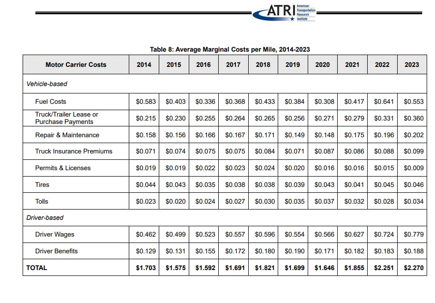
### Repair and Maintenance Cost - Heavy
Heavy truck maintenance costs come from industry surveys conducted by the American Transportation Research Institute (ATRI), which tracks operating costs for commercial trucking fleets. Maintenance costs include scheduled preventive maintenance (oil changes, filter replacements, inspections), repairs (brakes, tires, engine work), and roadside breakdowns. The data shows maintenance costs per mile ranging from $0.12 to $0.17, considerably higher than light-duty vehicle maintenance due to more frequent service intervals, larger and more expensive parts, and the severe duty cycles that commercial trucks experience.

Source: [TruckingInfo.com]('https://www.truckinginfo.com/10150350/2021-hdt-fact-book-maintenance-costs-expected-to-rise')
Source: [FleetMaintenance.com]('https://www.fleetmaintenance.com/equipment/article/55091624/atri-releases-2024-operational-costs-survey-report')
```{python}
# Set file path and source URL
filepath_truckops = Path("data/atri/parsed/ATRI-Operational-Costs-of-Trucking-07-2025.pdf")
url_truckops = "https://truckingresearch.org/wp-content/uploads/2025/07/ATRI-Operational-Costs-of-Trucking-07-2025.pdf"

# Ensure the file exists, Download if not
ensure_exists(path=filepath_truckops, url=url_truckops)
```
```{python}
# Manually Entering the data from above image
df_RepairMaintenanceCost_Heavy = pd.DataFrame({
    "Year": ["2010", "2011", "2012", "2013", "2014", "2015", "2016", "2017", "2018", "2019", "2020", "2021", "2022", "2023", "2024"],
    "CostMile": [0.124, 0.152, 0.138, 0.148, 0.158, 0.156, 0.166, 0.167, 0.171, 0.149, 0.148, 0.175, 0.196, 0.202, 0.198]
})

# display the data
df_RepairMaintenanceCost_Heavy
```
### Driving Costs
AAA publishes an annual "Your Driving Costs" report based on vehicle ownership costs for five vehicle categories at three annual mileage levels. The report combines manufacturer data, insurance industry statistics, and fuel price surveys. The PDF tables are extracted programmatically using `pdfplumber`, which identifies table boundaries and cell contents. The two pages are combined horizontally to create a complete dataset. This provides current-year cost estimates to benchmark against our trend-based calculations.
Data Source: [American Automobile Association]('https://exchange.aaa.com/wp-content/uploads/2019/09/AAA-Your-Driving-Costs-2019.pdf')
```{python}
# Set file path and source URL
filepath_drivingcost = Path("data/aaa/YDC-Brochure_2023-FINAL-8.30.23-.pdf")
url_drivingcost = "https://newsroom.aaa.com/wp-content/uploads/2023/08/YDC-Brochure_2023-FINAL-8.30.23-.pdf"

# Ensure the file exists, Download if not
ensure_exists(path=filepath_drivingcost, url=url_drivingcost)
```
```{python}
# Extract tables from PDF
tables_page1 = tabula.read_pdf(
  str(filepath_drivingcost),
  pages=1,
  multiple_tables=True,
  encoding='latin-1'  # or 'cp1252'
)

tables_page2 = tabula.read_pdf(
  str(filepath_drivingcost),
  pages=2,
  multiple_tables=True,
  encoding='latin-1'
)

# Get the first table from each page
df_page1 = tables_page1[0]
df_page2 = tables_page2[0]

# Remove the first column from df_page2 (equivalent to your drop operation)
df_page2_clean = df_page2.drop(df_page2.columns[0], axis=1)

# Concatenate horizontally
df_DrivingCosts = pd.concat([df_page1, df_page2_clean], axis=1)

df_DrivingCosts
```
## Intermediate Cost Calculations
Raw data alone cannot answer the question "what does it cost to drive a mile?" The data must be processed, combined, and analyzed to extract meaningful patterns and derive cost estimates. This section performs several types of calculations:
1. **Trend analysis:** Fitting linear regression lines to historical data to identify whether costs are rising, falling, or stable over time
2. **Data fusion:** Combining information from multiple sources (e.g., fuel prices from EIA and fuel economy from BTS to calculate fuel cost per mile)
3. **Actual vs. trend comparison:** Evaluating whether the most recent actual data point aligns with the long-term trend or represents an unusual deviation
4. **Normalization:** Adjusting costs for inflation using the CPI to enable valid comparisons across years
Each subsection focuses on a specific cost component, builds relevant metrics, visualizes trends, and produces comparison tables that inform the final operating cost calculations. The visualizations help both technical and non-technical readers understand whether recent costs are consistent with historical patterns or represent significant departures requiring explanation.
### Transportation Expenditures
Transportation expenditures provide essential context for validating our operating cost calculations. If our estimates are accurate, they should produce travel costs consistent with what households actually spend on transportation. This subsection examines transportation spending from two perspectives: transportation as a percentage of total household expenditures, and gasoline specifically as a percentage of total expenditures.
The first metric reveals how much of household budgets go to all transportation (vehicles, fuel, maintenance, public transit, air travel). The second isolates just gasoline, which directly relates to our per-mile operating cost estimates. If gasoline spending is rising faster than overall transportation spending, it suggests fuel prices are increasing or people are driving more. If it's falling, vehicles may be becoming more efficient or people may be driving less.
#### Create Dataframe
The dataframe combines transportation cost percentages from the personal expenditure data with gasoline costs from the average cost data. The calculation `Gasoline Cost of Transportation * Transportation Percent of Total / 100` produces gasoline as a percentage of total household expenditures. This derived metric helps us understand whether fluctuations in gasoline prices significantly impact household budgets or represent a small enough fraction that price changes have limited behavioral effects.
```{python}
#| eval: false
# Define year range
year_range = list(range(1990, BASE_YEAR+1)) # Last year should be one more than desired

# Ensure column names are strings in both DataFrames to avoid indexing issues
df_PersonalExpenditure.columns = df_PersonalExpenditure.columns.astype(str)
df_AverageCost.columns = df_AverageCost.columns.astype(str)

# Create a DataFrame to combine the extracted data
df_TransportationExpenditure = pd.DataFrame({
    # The years from 1990 to 2024
    "Year": year_range,
    # Extract the 'Transportation Cost Percent of Total' for the years 1990-2020 from row 2
    "Transportation Percent of Total": pd.to_numeric(
      df_PersonalExpenditure.loc[2, str(year_range[0]):str(year_range[-1])].values,
      errors="coerce"
    ),
    # Extract the 'Gasoline Cost of Transportation' for the years 1990-2020 from row 2
    "Gasoline Cost of Transportation": pd.to_numeric(
      df_AverageCost.loc[2, str(year_range[0]):str(year_range[-1])].values,
      errors="coerce"
    )
})

# FIXME: Did not understand the logic for this
df_TransportationExpenditure["Gasoline Percent of Total"] = df_TransportationExpenditure["Gasoline Cost of Transportation"] * df_TransportationExpenditure["Transportation Percent of Total"] / 100

df_TransportationExpenditure
```
#### Plotting Trends
The visualization shows two time series: the blue line represents all transportation spending as a percentage of total expenditures, while the red line shows just gasoline. Dashed trend lines reveal the long-term direction. Several insights emerge from these patterns:
* Transportation spending as a share of total expenditures has remained relatively stable at 12-13% over the 30+ year period, suggesting transportation is a consistent household priority
* Gasoline spending fluctuates more than total transportation spending, reflecting volatile oil prices
* When gasoline prices spike (visible as peaks in the red line), it absorbs a larger share of total transportation budgets, potentially crowding out other spending or changing travel behavior
* The gap between the lines represents non-gasoline transportation costs: vehicle purchases, insurance, maintenance, and public transit
```{python}
#| out-width: "100%"
#| eval: false
# Plotting the data using Seaborn and Matplotlib
# plt.figure(figsize=(10, 6))

# Plot Transportation Cost Percent of Total with a blue line
sns.lineplot(data=df_TransportationExpenditure, x='Year', y='Transportation Percent of Total',
             color='#0070C0', linewidth=2.5, label='Transportation as % of Total Expenditure')

# Plot Gasoline Percent of Total with a red line
sns.lineplot(data=df_TransportationExpenditure, x='Year', y='Gasoline Percent of Total',
             color='#FF0000', linewidth=2.5, label='Gasoline as % of Total Expenditure')

# Plotting the linear trend lines with dashed lines
sns.regplot(data=df_TransportationExpenditure, x='Year', y='Transportation Percent of Total',
            scatter=False, color='#0070C0', ci=None,
            line_kws={'linestyle': '--', 'linewidth': 2, 'alpha': 0.8})

sns.regplot(data=df_TransportationExpenditure, x='Year', y='Gasoline Percent of Total',
            scatter=False, color='#FF0000', ci=None,
            line_kws={'linestyle': '--', 'linewidth': 2, 'alpha': 0.8})

# Customize the plot
plt.title('Transportation as a Percent of Total Expenditure',
          fontsize=16, fontweight='bold', pad=20)
plt.xlabel('Year', fontsize=13)
plt.ylabel('% of Total Expenditure', fontsize=13)

# Show all x-axis labels with 90-degree rotation
plt.xticks(df_TransportationExpenditure['Year'], rotation=90)

plt.legend(loc='upper right', fontsize=11)

# Set y-axis limits to extend to 14
plt.ylim(0, 14)

# Add major and minor grid lines for better readability
plt.grid(True, alpha=0.3, linestyle='-', linewidth=0.5, which='major')

# Improve layout
plt.tight_layout()
plt.show()
```
#### Actual vs Trend Comparision
The comparison table evaluates whether 2023 values align with historical trends or deviate significantly. "Actual" shows the reported value from the data source for 2023. "Trend" shows the value predicted by a linear regression fit to all historical data.
Large differences between actual and trend values warrant investigation. If actual spending exceeds the trend, it might indicate unusual fuel price spikes or increased travel demand. If actual spending falls below the trend, it could reflect improved fuel economy, reduced travel, or fuel price declines. Small differences suggest stability and that using trend-based projections for missing data would be reasonable.
```{python}
#| eval: false
# Create the comparison DataFrame
df_TranspExp_Comparision = pd.DataFrame({
    'Date': [BASE_YEAR, BASE_YEAR],
    'Actual': [
        df_TransportationExpenditure.loc[df_TransportationExpenditure['Year'] == BASE_YEAR, 'Transportation Percent of Total'].iloc[0],
        df_TransportationExpenditure.loc[df_TransportationExpenditure['Year'] == BASE_YEAR, 'Gasoline Percent of Total'].iloc[0]  # FIXED: THere is a potential error here in Excel sheet
    ],
    'Trend': [
        np.poly1d(np.polyfit(pd.to_numeric(df_TransportationExpenditure['Year']),
                            pd.to_numeric(df_TransportationExpenditure['Transportation Percent of Total']), 1))(BASE_YEAR),
        np.poly1d(np.polyfit(pd.to_numeric(df_TransportationExpenditure['Year']),
                            pd.to_numeric(df_TransportationExpenditure['Gasoline Percent of Total']), 1))(BASE_YEAR)
    ]
}, index=['Transportation as % Total Expenditures', 'Gasoline as % Total Expenditures']).round(2)

df_TranspExp_Comparision
```
### Auto Cost - Variable-Fixed
Understanding the split between variable and fixed costs is fundamental to travel demand modeling. Variable costs—primarily fuel and maintenance—increase with each mile driven, so travelers experience them directly and may modify their behavior in response. Fixed costs—insurance, depreciation, registration, and finance charges—must be paid regardless of whether the vehicle is driven 5,000 or 25,000 miles per year.
Travel demand models typically include only variable costs because these represent the marginal cost of each trip. A traveler deciding whether to drive downtown doesn't consider their annual insurance premium (already paid) but does consider fuel and parking costs. By isolating variable costs and tracking how they've changed over time, we can better estimate the cost signals that influence travel decisions.
This section also normalizes costs by the Consumer Price Index to distinguish between nominal increases (due to general inflation) and real increases (costs rising faster than inflation). If variable costs increase faster than the CPI, driving is becoming genuinely more expensive in real terms, which may encourage modal shifts or trip consolidation.
#### Create Dataframe
The dataframe combines several cost components. "Variable" represents the cents-per-mile cost of fuel, maintenance, and tires—expenses that scale with mileage. "Fixed" represents annual costs for insurance, registration, depreciation, and finance charges. "Total" is the sum of variable and fixed costs.
The "Per 15k" column converts the annual fixed cost into a per-mile equivalent by dividing by 15,000 miles—the assumed annual travel in the AAA data. This allows direct comparison of fixed costs to variable costs on a per-mile basis, though it's important to remember this is an accounting convenience rather than a true marginal cost.
"Variable/Total" shows what fraction of total costs are variable—typically 30-40%. This indicates that most vehicle ownership costs are fixed commitments. "Variable/CPI" and "Fixed/CPI" divide costs by the Consumer Price Index to produce inflation-adjusted metrics. If these ratios increase over time, vehicle costs are rising faster than general inflation. If they decrease, vehicles are becoming relatively cheaper despite nominal price increases.
```{python}
#| eval: false
# Define year range
year_range = list(range(1990, BASE_YEAR+1))  # Last year should be one more than desired

# Compile data from Raw Datasets
df_AutoCost_VariableFixed = pd.DataFrame({
    "Year": year_range,
    "Variable": pd.to_numeric(
      df_AverageCost.loc[6, str(year_range[0]):str(year_range[-1])].values,
      errors="coerce"
    ),
    "Fixed": pd.to_numeric(
      df_AverageCost.loc[7, str(year_range[0]):str(year_range[-1])].values,
      errors="coerce"
    ),
    "Total": pd.to_numeric(
      df_AverageCost.loc[5, str(year_range[0]):str(year_range[-1])].values,
      errors="coerce"
    ),
    "CPI": pd.to_numeric(
      df_CPI[df_CPI['year'].between(year_range[0], year_range[-1])]["annualaverage"].values,
      errors="coerce"
    )
})

# Create Derived Columns
df_AutoCost_VariableFixed["Per 15k"] = df_AutoCost_VariableFixed["Fixed"] / 15000
df_AutoCost_VariableFixed["Variable/Total"] = df_AutoCost_VariableFixed["Variable"] / df_AutoCost_VariableFixed["Total"]
df_AutoCost_VariableFixed["Variable/CPI"] = df_AutoCost_VariableFixed["Variable"] / df_AutoCost_VariableFixed["CPI"]
df_AutoCost_VariableFixed["Fixed/CPI"] = df_AutoCost_VariableFixed["Fixed"] / df_AutoCost_VariableFixed["CPI"]

# Reorder columns
df_AutoCost_VariableFixed = df_AutoCost_VariableFixed[['Year', 'Variable/Total', 'Variable/CPI', 'Fixed/CPI', 'Variable', 'Fixed', 'Total', 'Per 15k', 'CPI']]

df_AutoCost_VariableFixed
```
#### Plotting Trends
##### Fixed/CPI and Variable/CPI
This chart normalizes both fixed and variable costs by the CPI to reveal real cost trends independent of general inflation. The smoothed spline curves reduce year-to-year noise to highlight underlying patterns.
The green line (Fixed/CPI) shows whether fixed ownership costs are rising or falling in real terms. A rising trend means insurance, depreciation, and registration costs are outpacing inflation. The red line (Variable/CPI) does the same for operating costs.
Notably, both series show considerable variation, reflecting the volatility of fuel prices (which dominate variable costs) and the episodic nature of insurance cost increases. The period from 2000-2010 saw rising real costs in both categories, while the 2010s showed some moderation. Understanding these patterns helps determine whether the base year represents typical conditions or an unusual outlier.
```{python}
#| out-width: "100%"
#| eval: false
# Plotting the data using Seaborn and Matplotlib
# plt.figure(figsize=(10, 6))

# Create smooth spline curves
x = df_AutoCost_VariableFixed['Year']
y_fixed = df_AutoCost_VariableFixed['Fixed/CPI']
y_variable = df_AutoCost_VariableFixed['Variable/CPI']

# Generate smooth curves
x_smooth = np.linspace(x.min(), x.max(), 300)
spline_fixed = make_interp_spline(x, y_fixed, k=3)
spline_variable = make_interp_spline(x, y_variable, k=3)

y_fixed_smooth = spline_fixed(x_smooth)
y_variable_smooth = spline_variable(x_smooth)

# Plot smooth lines
sns.lineplot(x=x_smooth, y=y_fixed_smooth, linewidth=2.5, color="#00B050", label="Fixed/CPI")
sns.lineplot(x=x_smooth, y=y_variable_smooth, linewidth=2.5, color="#FF0000", label="Variable/CPI")

# Format y-axis as currency with comma separation using anonymous function
plt.gca().yaxis.set_major_formatter(FuncFormatter(lambda x, p: f'${x:,.0f}'))

# Customize the plot
plt.title('Trendline of Fixed/CPI and Variable/CPI (1990–2020)',
          fontsize=16, fontweight='bold', pad=20)
plt.xlabel('Year', fontsize=13)
plt.ylabel('Value', fontsize=13)

# Show all x-axis labels with 90-degree rotation
plt.xticks(df_AutoCost_VariableFixed['Year'], rotation=90)

plt.legend(loc='upper right', fontsize=11)

# Set y-axis limits to extend to $40
plt.ylim(0, 40)

# Add major and minor grid lines for better readability
plt.grid(True, alpha=0.3, linestyle='-', linewidth=0.5, which='major')

# Improve layout
plt.tight_layout()
plt.show()
```
##### Average Cost per Mile
This stacked area chart visualizes the composition of total vehicle costs. The green area represents fixed costs, while the red area shows variable costs stacked on top. The total height at any year represents the total cost per 15,000 miles.
Several patterns emerge:
* Total costs have increased over time, rising from around $4,000 in 1990 to $9,000+ in recent years
* Variable costs (red) fluctuate more than fixed costs, visible in the undulating upper boundary
* Fixed costs (green) grow more steadily, reflecting consistent increases in insurance premiums and vehicle prices
* The variable cost portion occasionally spikes, particularly during periods of high oil prices (mid-2000s, early 2010s)
The chart provides intuitive visual confirmation of the trend analysis while making the relative magnitudes immediately apparent to non-technical readers.
```{python}
#| out-width: "100%"
#| eval: false
# Create the stacked area plot
# plt.figure(figsize=(10, 6))

# Stack the areas - Fixed on bottom, Variable on top
plt.fill_between(df_AutoCost_VariableFixed['Year'],
                 0,
                 df_AutoCost_VariableFixed['Fixed'],
                 color='#9BBB59',
                 label='Fixed')

plt.fill_between(df_AutoCost_VariableFixed['Year'],
                 df_AutoCost_VariableFixed['Fixed'],
                 df_AutoCost_VariableFixed['Fixed'] + df_AutoCost_VariableFixed['Variable'],
                 color='#C0504D',
                 label='Variable')

# Format y-axis as currency with comma separation using anonymous function
plt.gca().yaxis.set_major_formatter(FuncFormatter(lambda x, p: f'${x:,.0f}'))

# Customize the plot
plt.title('Average Total Cost per 15,000 Miles',
          fontsize=16, fontweight='bold', pad=20)
plt.xlabel('Year', fontsize=13)
plt.ylabel('USDs', fontsize=13)

# Show all x-axis labels with 90-degree rotation
plt.xticks(df_AutoCost_VariableFixed['Year'], rotation=90)

plt.legend(loc='upper left', fontsize=11)

# Set y-axis limits
plt.ylim(bottom=0)

# Add grid
plt.grid(True, alpha=0.3, linestyle='-', linewidth=0.5, which='major')

# Improve layout
plt.tight_layout()
plt.show()
```
#### Actual vs Trend Comparision
This comparison assesses whether 2023 costs align with long-term trends. Each row compares the actual value from the AAA data against the predicted value from a linear trend fit to 1990-2023 data.
"Variable" costs show whether fuel and maintenance in 2023 are higher or lower than historical patterns would predict. Given the volatility of fuel prices, some deviation is expected. Large positive deviations suggest an unusually expensive year, while negative deviations indicate relative affordability.
"Fixed" costs are typically more stable, so large deviations are less common. "Fixed per 15,000 Miles" converts annual fixed costs to a per-mile basis for comparison purposes, though remember this is not a true marginal cost.
Analysts should investigate any large discrepancies. If actual costs substantially exceed trends, using trend-based estimates might understate current costs. If actual costs fall well below trends, it might signal a structural change in the market or data collection methodology.
```{python}
#| eval: false
# Create the comparison DataFrame
df_AutoCost_VariableFixed_Comparision = pd.DataFrame({
    'Date': [BASE_YEAR, BASE_YEAR, BASE_YEAR],
    'Actual': [
        df_AutoCost_VariableFixed.loc[df_AutoCost_VariableFixed['Year'] == BASE_YEAR, 'Variable'].iloc[0],
        df_AutoCost_VariableFixed.loc[df_AutoCost_VariableFixed['Year'] == BASE_YEAR, 'Fixed'].iloc[0],
        df_AutoCost_VariableFixed.loc[df_AutoCost_VariableFixed['Year'] == BASE_YEAR, 'Per 15k'].iloc[0]
    ],
    'Trend': [
        np.poly1d(np.polyfit(pd.to_numeric(df_AutoCost_VariableFixed['Year']),
                            pd.to_numeric(df_AutoCost_VariableFixed['Variable']), 1))(BASE_YEAR),
        np.poly1d(np.polyfit(pd.to_numeric(df_AutoCost_VariableFixed['Year']),
                            pd.to_numeric(df_AutoCost_VariableFixed['Fixed']), 1))(BASE_YEAR),
        np.poly1d(np.polyfit(pd.to_numeric(df_AutoCost_VariableFixed['Year']),
                            pd.to_numeric(df_AutoCost_VariableFixed['Per 15k']), 1))(BASE_YEAR)
    ]
}, index=['Variable', 'Fixed', 'Fixed per 15,000 Miles']).round(2)

df_AutoCost_VariableFixed_Comparision
```
### Auto Cost
This subsection isolates the two primary variable cost components that appear in travel demand models: fuel costs and maintenance-plus-tires. While the previous section examined total variable costs, here we separate gasoline specifically from other variable expenses.
Fuel costs respond directly to oil markets and refinery economics. Maintenance and tire costs respond to vehicle reliability, parts prices, and labor rates. By analyzing these separately, we can identify which component drives changes in total variable costs and assess whether they move together or independently.
This disaggregation also allows us to construct operating costs from first principles: calculating fuel cost per mile (price per gallon ÷ miles per gallon) and adding maintenance cost per mile. This bottom-up approach provides more transparency than using aggregated cost figures.
#### Create Dataframe
The dataframe extracts three series from the AAA average cost data: "Gas" (the cents-per-mile fuel cost), "Maint" (maintenance cost per mile), and "Tires" (tire cost per mile). In some years, maintenance and tires are reported separately; in others, they're combined. The code uses `.fillna(0)` to handle missing values, ensuring that when only one value is present, the sum still works correctly.
"Maint+Tires" combines these two closely related costs. Both represent wear-and-tear expenses that scale with mileage. Maintenance includes oil changes, brake replacements, and routine service. Tires wear out with miles driven and must be replaced periodically. Together, they represent the non-fuel variable costs of driving.
```{python}
# Define year range
year_range = list(range(1990, BASE_YEAR+1)) # Last year should be one more than desired

# Compile data from Raw Datasets
df_AutoCost = pd.DataFrame({
    "Year": year_range,
    "Gas": pd.to_numeric(
        df_AverageCost.loc[1, str(year_range[0]):str(year_range[-1])].values,
        errors="coerce"
    ),
    "Maint": pd.to_numeric(
        df_AverageCost.loc[3, str(year_range[0]):str(year_range[-1])].values,
        errors="coerce"
    ),
    "Tires": pd.to_numeric(
        df_AverageCost.loc[4, str(year_range[0]):str(year_range[-1])].values,
        errors="coerce"   # turns "U" into NaN
    )
})

df_AutoCost["Maint+Tires"] = df_AutoCost["Maint"].fillna(0) + df_AutoCost["Tires"].fillna(0)

# View Dataframe
df_AutoCost
```
#### Plotting Trends
The visualization compares fuel costs (blue line) with maintenance-plus-tires costs (red line). Dashed trend lines show the long-term trajectory of each component.
Key observations:
* Fuel costs (blue) are consistently higher than maintenance costs and show more volatility, reflecting oil price fluctuations
* Maintenance costs (red) increase gradually over time, likely driven by parts price inflation and increasing vehicle complexity
* The gap between the lines varies with fuel prices—during high oil price periods, fuel costs can be 2-3 times maintenance costs
* Both show upward trends, but fuel costs rise more steeply, meaning fuel is becoming a larger fraction of variable costs
The trend lines provide predicted values for the base year that smooth out year-to-year fluctuations. If 2023 data points fall close to trend lines, using trend-based estimates is justified. Large deviations suggest the need to use actual values or investigate the causes of unusual costs.
```{python}
#| out-width: "100%"
# Plotting the data using Seaborn and Matplotlib
# plt.figure(figsize=(10, 6))

# Plot Fixed/CPI with a green line
sns.lineplot(data=df_AutoCost, x="Year", y="Gas",
linewidth=2.5, color="#0070C0", label="Gas")

# Plot Variable/CPI with a red line
sns.lineplot(data=df_AutoCost, x="Year", y="Maint+Tires",
linewidth=2.5,color="#FF0000", label="Maint+Tires")

# Plotting the linear trend lines with dashed lines
sns.regplot(data=df_AutoCost, x='Year', y='Gas',
            scatter=False, color='#0070C0', ci=None,
            line_kws={'linestyle': '--', 'linewidth': 2, 'alpha': 0.8})

sns.regplot(data=df_AutoCost, x='Year', y='Maint+Tires',
            scatter=False, color='#FF0000', ci=None,
            line_kws={'linestyle': '--', 'linewidth': 2, 'alpha': 0.8})

# Format y-axis as currency with comma separation using anonymous function
plt.gca().yaxis.set_major_formatter(FuncFormatter(lambda x, p: f'${x:,.2f}'))

# Customize the plot
plt.title('Average Auto Costs',
          fontsize=16, fontweight='bold', pad=20)
plt.xlabel('Year', fontsize=13)
plt.ylabel('USDs', fontsize=13)

# Show all x-axis labels with 90-degree rotation
plt.xticks(df_AutoCost['Year'], rotation=90)

plt.legend(loc='upper left', fontsize=11)

# Set y-axis limits
plt.ylim(bottom=0)

# Add major and minor grid lines for better readability
plt.grid(True, alpha=0.3, linestyle='-', linewidth=0.5, which='major')

# Improve layout
plt.tight_layout()
plt.show()
```
#### Actual vs Trend Comparision
This table compares 2023 actual costs against trend predictions for both fuel and maintenance-plus-tires.
The "Gas" row reveals whether fuel prices in 2023 are high or low relative to the long-term trend. Fuel markets are volatile, so moderate deviations are normal. Large deviations might reflect temporary supply disruptions, geopolitical events, or unusual demand conditions.
The "Maint+Tires" row is typically more stable. Significant deviations here might indicate changes in vehicle reliability (newer vehicles requiring less maintenance), shifts in labor costs, or changes in how AAA calculates these figures.
For travel demand models, using trend values rather than actual values can be justified when actual values represent temporary anomalies. However, if the deviation persists across multiple years, it may signal a structural shift requiring adjustment to the model.
```{python}
# Create the comparison DataFrame
df_AutoCost_Comparision = pd.DataFrame({
    'Date': [BASE_YEAR, BASE_YEAR],
    'Actual': [
        df_AutoCost.loc[df_AutoCost['Year'] == BASE_YEAR, 'Gas'].iloc[0],
        df_AutoCost.loc[df_AutoCost['Year'] == BASE_YEAR, 'Maint+Tires'].iloc[0]
    ],
    'Trend': [
        np.poly1d(np.polyfit(pd.to_numeric(df_AutoCost['Year']),
                            pd.to_numeric(df_AutoCost['Gas']), 1))(BASE_YEAR),
        np.poly1d(np.polyfit(pd.to_numeric(df_AutoCost['Year']),
                            pd.to_numeric(df_AutoCost['Maint+Tires']), 1))(BASE_YEAR)
    ]
}, index=['Gas', 'Maint+Tires']).round(2)

df_AutoCost_Comparision
```
### Vehicle Miles - Trucks
Average annual vehicle miles traveled (VMT) varies dramatically by truck class. Light trucks (pickups and SUVs used for personal travel) typically drive 10,000-15,000 miles per year. Medium trucks (delivery vehicles) might drive 15,000-25,000 miles. Heavy trucks (long-haul tractor-trailers) often exceed 60,000 miles annually.
Understanding these patterns serves two purposes. First, it helps calibrate whether our fuel economy and cost estimates are reasonable—a vehicle class with unusually high or low VMT should have corresponding impacts on total fuel consumption. Second, it informs how we weight different vehicle classes when calculating fleet-average statistics.
This subsection tracks trends in truck VMT over time. Are trucks driving more miles as the economy grows and freight demand increases? Are efficiency improvements or modal shifts reducing truck VMT? The analysis looks at both the full 1990-2023 period and a 2000-2023 subset to check whether recent trends differ from long-term patterns.
#### Create Dataframe
The dataframe compiles average annual VMT for three truck categories. "Heavy" refers to combination trucks—tractor-trailers used for long-haul freight. "Medium" covers single-unit trucks—delivery vehicles, utility trucks, and other medium-duty applications. "Light" includes pickup trucks and SUVs primarily used for personal transportation or light commercial purposes.
The data comes from BTS tables that compile Federal Highway Administration statistics on vehicle registration, fuel consumption, and estimated miles traveled. Dividing total miles by number of vehicles yields average VMT per vehicle. These are fleet-wide averages; individual vehicles may drive considerably more or less depending on their specific usage patterns.
```{python}
#| eval: false
# Define year range
year_range = list(range(1990, BASE_YEAR+1)) # Last year should be one more than desired

# Ensure column names are strings in both DataFrames to avoid indexing issues
df_FE_Heavy.columns = df_FE_Heavy.columns.astype(str)
df_FE_Medium.columns = df_FE_Medium.columns.astype(str)
df_4_11.columns = df_4_11.columns.astype(str)

# Compile data from Raw Datasets
df_VehicleMiles_Truck = pd.DataFrame({
  "Year": year_range,
  "Heavy": pd.to_numeric(
    df_FE_Heavy.loc[3, str(year_range[0]):str(year_range[-1])].values,
    errors="coerce"
  ),
  "Medium": pd.to_numeric(
    df_FE_Medium.loc[3, str(year_range[0]):str(year_range[-1])].values,
    errors="coerce"
  ),
  "Light": pd.to_numeric(
    df_4_11.loc[10, str(year_range[0]):str(year_range[-1])].values,
    errors="coerce"
  )
})

# View dataframe
df_VehicleMiles_Truck
```
#### Plotting Trends
##### 1990 - 2023
This chart shows VMT trends for all three truck classes over the full data period. The blue line (Heavy) shows that long-haul trucks average 50,000-70,000 miles per year with a generally flat trend—these vehicles are already used intensively, and there's limited room for further increases. The red line (Medium) shows medium trucks traveling 12,000-16,000 miles annually with moderate growth, reflecting increased delivery activity. The green line (Light) shows light trucks at 11,000-13,000 miles per year, similar to passenger cars.
Only the heavy truck trend line is shown here (dashed blue) to avoid visual clutter, as it's the most stable series. The relatively flat trend for heavy trucks suggests that regulatory limits on driver hours and the physical constraints of long-haul trucking have kept average VMT stable even as total freight volumes have grown (accommodated by adding more trucks rather than driving each truck further).
```{python}
#| out-width: "100%"
#| eval: false
# Plotting the data using Seaborn and Matplotlib
# plt.figure(figsize=(10, 6))

# Plot Variable with a red line
sns.lineplot(data=df_VehicleMiles_Truck, x="Year", y="Heavy",
linewidth=2.5,color="#0070C0", label="Heavy")

# Plot Variable with a red line
sns.lineplot(data=df_VehicleMiles_Truck, x="Year", y="Medium",
linewidth=2.5,color="#BE4B48", label="Medium")

# Plot Fixed with a green line
sns.lineplot(data=df_VehicleMiles_Truck, x="Year", y="Light",
linewidth=2.5, color="#98B954", label="Light")

# Plotting the linear trend lines with dashed lines
sns.regplot(data=df_VehicleMiles_Truck, x='Year', y='Heavy',
            scatter=False, color='#0070C0', ci=None,
            line_kws={'linestyle': '--', 'linewidth': 2, 'alpha': 0.8})

# Customize the plot
plt.title('Average Vehicle Miles - Trucks (1990 - 2023)',
          fontsize=16, fontweight='bold', pad=20)
plt.xlabel('Year', fontsize=13)
plt.ylabel('Miles', fontsize=13)

# Show all x-axis labels with 90-degree rotation
plt.xticks(df_VehicleMiles_Truck['Year'], rotation=90)

plt.legend(loc='upper right', fontsize=11)

# Set y-axis limits to extend to 80
plt.ylim(0, 80)

# Add major and minor grid lines for better readability
plt.grid(True, alpha=0.3, linestyle='-', linewidth=0.5, which='major')

# Improve layout
plt.tight_layout()
plt.show()
```
##### 2000 - 2023
This chart focuses on the more recent period to check whether trends have changed. All three trend lines are now shown (dashed).
Comparing to the 1990-2023 chart reveals that light and medium truck VMT patterns changed around 2000. The 2000+ trends show slight increases for medium trucks (driven by e-commerce growth and more frequent deliveries) and slight decreases for light trucks (possibly reflecting higher fuel prices making owners more selective about trip-making).
Heavy truck VMT remains remarkably stable across both time periods, confirming that these vehicles are operated at maximum intensity regardless of economic conditions. This stability makes heavy truck operating costs particularly sensitive to fuel price changes—operators cannot significantly reduce miles to offset higher fuel costs.
```{python}
#| out-width: "100%"
#| eval: false
# Plotting the data using Seaborn and Matplotlib
# plt.figure(figsize=(10, 6))

# Plot Variable with a red line
sns.lineplot(data=df_VehicleMiles_Truck, x="Year", y="Heavy",
linewidth=2.5,color="#0070C0", label="Heavy")

# Plot Variable with a red line
sns.lineplot(data=df_VehicleMiles_Truck, x="Year", y="Medium",
linewidth=2.5,color="#BE4B48", label="Medium")

# Plot Fixed with a green line
sns.lineplot(data=df_VehicleMiles_Truck, x="Year", y="Light",
linewidth=2.5, color="#00B050", label="Light")

# Plotting the linear trend lines with dashed lines
sns.regplot(data=df_VehicleMiles_Truck, x='Year', y='Heavy',
            scatter=False, color='#0070C0', ci=None,
            line_kws={'linestyle': '--', 'linewidth': 2, 'alpha': 0.8})

# Plotting the linear trend lines with dashed lines
sns.regplot(data=df_VehicleMiles_Truck, x='Year', y='Medium',
            scatter=False, color='#FF0000', ci=None,
            line_kws={'linestyle': '--', 'linewidth': 2, 'alpha': 0.8})

# Plotting the linear trend lines with dashed lines
sns.regplot(data=df_VehicleMiles_Truck, x='Year', y='Light',
            scatter=False, color='#00B050', ci=None,
            line_kws={'linestyle': '--', 'linewidth': 2, 'alpha': 0.8})

# Customize the plot
plt.title('Average Vehicle Miles - Trucks (2000 - 2023)',
          fontsize=16, fontweight='bold', pad=20)
plt.xlabel('Year', fontsize=13)
plt.ylabel('Miles', fontsize=13)

# Show all x-axis labels with 90-degree rotation
plt.xticks(df_VehicleMiles_Truck['Year'], rotation=90)

plt.legend(loc='upper right', fontsize=11)

# Set x-axis limits to show only 2000-2023
plt.xlim(2000, BASE_YEAR)

# Set y-axis limits to extend to 80
plt.ylim(0, 80)

# Add major and minor grid lines for better readability
plt.grid(True, alpha=0.3, linestyle='-', linewidth=0.5, which='major')

# Improve layout
plt.tight_layout()
plt.show()
```
#### Actual vs Trend Comparision
This comparison table shows 2023 VMT estimates using two different trend periods: 1990-2023 and 2000-2023.
The first three rows use the full data period. The second three rows use only post-2000 data. Comparing these reveals whether recent trends differ from long-term patterns. If the two trend estimates are similar, it suggests stable, consistent behavior. Large differences indicate a structural break around 2000, making recent trends more relevant for current-year estimates.
For heavy trucks, both approaches yield similar results, confirming the stability of this market segment. For light and medium trucks, the estimates may differ more, reflecting the changing roles of these vehicles in the economy. Medium truck VMT has likely increased with e-commerce growth, while light truck VMT may have declined as fuel economy concerns limited discretionary driving.
```{python}
#| eval: false
# Create the comparison DataFrame
df_VMTrucks_Comparision = pd.DataFrame({
    'Date': [BASE_YEAR, BASE_YEAR, BASE_YEAR, BASE_YEAR, BASE_YEAR, BASE_YEAR],
    'Actual': [
        df_VehicleMiles_Truck.loc[df_VehicleMiles_Truck['Year'] == BASE_YEAR, 'Heavy'].iloc[0],
        df_VehicleMiles_Truck.loc[df_VehicleMiles_Truck['Year'] == BASE_YEAR, 'Medium'].iloc[0],
        df_VehicleMiles_Truck.loc[df_VehicleMiles_Truck['Year'] == BASE_YEAR, 'Light'].iloc[0],
        df_VehicleMiles_Truck.loc[df_VehicleMiles_Truck['Year'] == BASE_YEAR, 'Heavy'].iloc[0],
        df_VehicleMiles_Truck.loc[df_VehicleMiles_Truck['Year'] == BASE_YEAR, 'Medium'].iloc[0],
        df_VehicleMiles_Truck.loc[df_VehicleMiles_Truck['Year'] == BASE_YEAR, 'Light'].iloc[0]
    ],
    'Trend': [
        np.poly1d(np.polyfit(pd.to_numeric(df_VehicleMiles_Truck['Year']),
                            pd.to_numeric(df_VehicleMiles_Truck['Heavy']), 1))(BASE_YEAR),
        np.poly1d(np.polyfit(pd.to_numeric(df_VehicleMiles_Truck['Year']),
                            pd.to_numeric(df_VehicleMiles_Truck['Medium']), 1))(BASE_YEAR),
        np.poly1d(np.polyfit(pd.to_numeric(df_VehicleMiles_Truck['Year']),
                            pd.to_numeric(df_VehicleMiles_Truck['Light']), 1))(BASE_YEAR),
        # Last 3: Use only data from 2000+
        np.poly1d(np.polyfit(
          pd.to_numeric(df_VehicleMiles_Truck[df_VehicleMiles_Truck['Year'] >= 2000]['Year']),
          pd.to_numeric(df_VehicleMiles_Truck[df_VehicleMiles_Truck['Year'] >= 2000]['Heavy']), 1))(BASE_YEAR),
        np.poly1d(np.polyfit(
          pd.to_numeric(df_VehicleMiles_Truck[df_VehicleMiles_Truck['Year'] >= 2000]['Year']),
          pd.to_numeric(df_VehicleMiles_Truck[df_VehicleMiles_Truck['Year'] >= 2000]['Medium']), 1))(BASE_YEAR),
        np.poly1d(np.polyfit(
          pd.to_numeric(df_VehicleMiles_Truck[df_VehicleMiles_Truck['Year'] >= 2000]['Year']),
          pd.to_numeric(df_VehicleMiles_Truck[df_VehicleMiles_Truck['Year'] >= 2000]['Light']), 1))(BASE_YEAR)
    ]
}, index=['Heavy Trucks  - 1990+', 'Medium Trucks  - 1990+', 'Light Trucks  - 1990+',
'Heavy Trucks  - 2000+', 'Medium Trucks  - 2000+', 'Light Trucks  - 2000+']).round(2)

# TODO: '1980+' should be changed to '1990+'

df_VMTrucks_Comparision
```
### Fuel Economy
Fuel economy—miles traveled per gallon of fuel consumed—directly determines fuel costs per mile. A vehicle that achieves 25 miles per gallon at $3.00/gallon costs $0.12 per mile for fuel. One that achieves only 6 miles per gallon costs $0.50 per mile—more than four times as much.
Fuel economy has improved substantially over time due to technological advances (better engines, transmissions, aerodynamics) and regulatory pressure (CAFE standards for cars and light trucks, fuel economy standards for heavy trucks). However, improvements vary by vehicle class. Light-duty vehicles have seen dramatic gains, rising from under 20 mpg in the 1980s to over 25 mpg today. Heavy trucks have improved more modestly, from 5.5 to 6.5 mpg, because the physics of moving heavy loads limits efficiency gains.
This subsection tracks fuel economy trends for three vehicle classes: light-duty (cars and small SUVs), medium-duty (delivery trucks), and heavy-duty (tractor-trailers). By comparing actual 2023 fuel economy against long-term trends, we can assess whether recent values are typical or represent unusual efficiency improvements or setbacks.
#### Create Dataframe
The dataframe compiles fuel economy data for three truck/vehicle categories spanning 1980-2023. The year range starts earlier than other series (1980 and 1985 are included) to capture the full arc of fuel economy improvement following the oil crises of the 1970s.
"Light Duty" comes from BTS Table 4-23, which tracks average fuel economy of the U.S. light-duty vehicle fleet—both cars and light trucks weighted by their share of vehicle miles traveled. This represents actual on-road fuel economy, which is typically 20-25% lower than EPA test ratings due to aggressive driving, air conditioning use, cold starts, and other real-world factors.
"Medium Duty" and "Heavy Duty" come from BTS tables on single-unit and combination trucks. These are calculated by dividing total miles traveled by total fuel consumed for each truck class. Note that a calculation error in the original analysis has been corrected—the code now properly extracts fuel economy (row 4) rather than fuel consumption (row 5).
```{python}
# Define year range
year_range = [1980, 1985] + list(range(1990, BASE_YEAR+1)) # Last year of the range should be one more than desired

# Ensure column names are strings in both DataFrames to avoid indexing issues
df_FE_LightDuty.columns = df_FE_LightDuty.columns.astype(str)
df_FE_Medium.columns = df_FE_Medium.columns.astype(str)
df_FE_Heavy.columns = df_FE_Heavy.columns.astype(str)

# Compile data from Raw Datasets
df_FuelEconomy = pd.DataFrame({
  "Year": year_range,
  "Light Duty": pd.to_numeric(
    df_FE_LightDuty.loc[0, str(year_range[0]):str(year_range[-1])].values,
    errors="coerce"
  ),
  "Medium Duty": pd.to_numeric(
    df_FE_Medium.loc[4, str(year_range[0]):str(year_range[-1])].values, # FIXED: Mistake in original calculation; use this instead
    errors="coerce"
  ),
  "Heavy Duty": pd.to_numeric(
    df_FE_Heavy.loc[4, str(year_range[0]):str(year_range[-1])].values, # FIXED: Mistake in original calculation; use this instead
    errors="coerce"
  )
})

# View the dataset
df_FuelEconomy
```
#### Plotting Trends
This chart shows fuel economy trends for all three vehicle classes with trend lines. Several important patterns emerge:
* The blue line (Light Duty) shows substantial improvement, rising from about 16 mpg in 1980 to over 24 mpg by 2023. This reflects CAFE standards requiring manufacturers to improve fleet fuel economy, along with technological improvements like direct fuel injection, turbocharging, continuously variable transmissions, and cylinder deactivation. The trend is approximately linear, suggesting consistent progress over time.
* The red line (Medium Duty) shows more modest improvement, from about 6.5 to 8 mpg. Medium trucks face conflicting pressures: efficiency improvements versus increasing vehicle size and capability. The trend is flatter than light-duty, indicating slower progress.
* The green line (Heavy Duty) is flattest of all, improving from about 5.5 to 6.0 mpg. Heavy truck fuel economy is limited by fundamental physics—aerodynamic drag and rolling resistance of a 80,000-pound vehicle. Recent regulations requiring aerodynamic improvements (side skirts, trailer tails) and low-rolling-resistance tires have helped, but gains are incremental.
The trend lines provide expected 2023 values that smooth out year-to-year variation from weather, economic conditions, and data collection variability.
```{python}
#| out-width: "100%"
# Plotting the data using Seaborn and Matplotlib
# plt.figure(figsize=(10, 6))

# Plot Variable with a red line
sns.lineplot(data=df_FuelEconomy, x="Year", y="Light Duty",
linewidth=2.5,color="#0070C0", label="Light Duty")

# Plot Variable with a red line
sns.lineplot(data=df_FuelEconomy, x="Year", y="Medium Duty",
linewidth=2.5,color="#FF0000", label="Medium Duty")

# Plot Fixed with a green line
sns.lineplot(data=df_FuelEconomy, x="Year", y="Heavy Duty",
linewidth=2.5, color="#00B050", label="Heavy Duty")

# Plotting the linear trend lines with dashed lines
sns.regplot(data=df_FuelEconomy, x='Year', y='Light Duty',
            scatter=False, color='#0070C0', ci=None,
            line_kws={'linestyle': '--', 'linewidth': 2, 'alpha': 0.8})

# Plotting the linear trend lines with dashed lines
sns.regplot(data=df_FuelEconomy, x='Year', y='Medium Duty',
            scatter=False, color='#FF0000', ci=None,
            line_kws={'linestyle': '--', 'linewidth': 2, 'alpha': 0.8})

# Plotting the linear trend lines with dashed lines
sns.regplot(data=df_FuelEconomy, x='Year', y='Heavy Duty',
            scatter=False, color='#00B050', ci=None,
            line_kws={'linestyle': '--', 'linewidth': 2, 'alpha': 0.8})

# Format y-axis as currency with comma separation using anonymous function
plt.gca().yaxis.set_major_formatter(FuncFormatter(lambda x, p: f'${x:,.2f}'))

# Customize the plot
plt.title('Average Fuel Economy (miles per gallon)',
          fontsize=16, fontweight='bold', pad=20)
plt.xlabel('Year', fontsize=13)
plt.ylabel('Miles Travelled per Gallon', fontsize=13)

# Show all x-axis labels with 90-degree rotation
plt.xticks(df_FuelEconomy['Year'], rotation=90)

plt.legend(loc='upper left', fontsize=11)

# Set y-axis limits to extend to 25
plt.ylim(0, 25)

# Add major and minor grid lines for better readability
plt.grid(True, alpha=0.3, linestyle='-', linewidth=0.5, which='major')

# Improve layout
plt.tight_layout()
plt.show()
```
#### Actual vs Trend Comparision
This table compares actual 2023 fuel economy against trend-based predictions for each vehicle class.
The "Light Duty" comparison reveals whether recent improvements in passenger vehicle efficiency are ahead of, behind, or on track with the long-term trend. If actual values exceed the trend, it might reflect a particularly good year for fuel economy—perhaps high gas prices encouraged purchasing more efficient vehicles. If actual values fall below the trend, it could indicate a shift toward larger vehicles or more aggressive driving.
"Medium Duty" and "Heavy Duty" comparisons are similarly revealing. These markets respond less to consumer preferences and more to regulatory requirements and operational economics. Fleet operators maximize efficiency to reduce fuel costs, so deviations from trend likely reflect regulatory changes or technological breakthroughs rather than behavioral shifts.
For operating cost calculations, using trend values is generally appropriate for fuel economy because these represent long-term technological capability rather than short-term market fluctuations. However, if actual values consistently exceed trends for several years, it may indicate a structural improvement worth incorporating.
```{python}
# Create the comparison DataFrame
df_FuelEconomy_Comparision = pd.DataFrame({
    'Date': [BASE_YEAR, BASE_YEAR, BASE_YEAR],
    'Actual': [
        df_FuelEconomy.loc[df_FuelEconomy['Year'] == BASE_YEAR, 'Light Duty'].iloc[0],
        df_FuelEconomy.loc[df_FuelEconomy['Year'] == BASE_YEAR, 'Medium Duty'].iloc[0],
        df_FuelEconomy.loc[df_FuelEconomy['Year'] == BASE_YEAR, 'Heavy Duty'].iloc[0]
    ],
    'Trend': [
        np.poly1d(np.polyfit(pd.to_numeric(df_FuelEconomy['Year']),
                            pd.to_numeric(df_FuelEconomy['Light Duty']), 1))(BASE_YEAR),
        np.poly1d(np.polyfit(pd.to_numeric(df_FuelEconomy['Year']),
                            pd.to_numeric(df_FuelEconomy['Medium Duty']), 1))(BASE_YEAR),
        np.poly1d(np.polyfit(pd.to_numeric(df_FuelEconomy['Year']),
                            pd.to_numeric(df_FuelEconomy['Heavy Duty']), 1))(BASE_YEAR)
    ]
}, index=['Light Duty', 'Medium Duty', 'Heavy Duty']).round(2)

df_FuelEconomy_Comparision
```
### Fuel Costs
Fuel prices are the most volatile component of vehicle operating costs. Unlike fuel economy (which changes gradually with fleet turnover) or maintenance costs (which increase slowly with parts and labor inflation), fuel prices can swing 50% or more in a single year due to crude oil markets, refinery outages, geopolitical events, and seasonal demand patterns.
Regional variations in fuel prices also matter. The Rocky Mountain region (which includes Utah) typically has prices 5-15% different from the national average due to distance from refineries, pipeline capacity constraints, and regional fuel formulation requirements. Using region-specific prices improves the accuracy of operating cost estimates for our study area.
This subsection compiles daily fuel price data for both gasoline and diesel in the Rocky Mountain region from 1994 through 2024. We analyze both the full 30-year period and a more recent 20-year window (2005-2024) to assess whether long-term trends differ from recent patterns. This is particularly important given the oil price spike of 2008, the collapse in 2014-2016, and the 2020-2022 pandemic-related volatility.
#### Create Dataframe
The dataframe merges gasoline and diesel price series into a single time series dataset spanning 1994-2024. The EIA publishes weekly prices, but we match them to a daily date range to enable precise date-based lookups.
"Gasoline $/gal" contains the retail price for all grades of gasoline in the Rocky Mountain region. This is a volume-weighted average of regular, midgrade, and premium grades reflecting actual consumer purchases. About 85% of gasoline sold is regular grade.
"Diesel $/gal" contains the retail price for on-highway diesel fuel (No. 2 diesel) in the Rocky Mountain region. This is the fuel type used by medium and heavy trucks. Off-highway diesel (used in agriculture and construction) has lower taxes and is not included.
Missing values appear as NaN (Not a Number). These typically occur in the first few years when diesel price reporting was less comprehensive. The code handles these properly by dropping NaN values before fitting trend lines.
```{python}
# Generate the date range between the desired dates
date_range = pd.date_range("1994-01-03", "2024-12-31", freq="D")

# Compile data from Raw Datasets
df_FuelCosts = pd.DataFrame({
  "Date": df_RetailGasPrices[df_RetailGasPrices['Date'].isin(date_range)]['Date'].values
})

# Merge Gasoline and Diesel prices directly
df_FuelCosts = df_FuelCosts.merge(df_RetailGasPrices[['Date', 'Weekly Rocky Mountain All Grades All Formulations Retail Gasoline Prices  (Dollars per Gallon)']], on='Date', how='left') \
                            .merge(df_RetailDieselPrices[['Date', 'Weekly Rocky Mountain No 2 Diesel Retail Prices  (Dollars per Gallon)']], on='Date', how='left')

# Rename columns
df_FuelCosts.rename(columns={
    'Weekly Rocky Mountain All Grades All Formulations Retail Gasoline Prices  (Dollars per Gallon)': 'Gasoline $/gal',
    'Weekly Rocky Mountain No 2 Diesel Retail Prices  (Dollars per Gallon)': 'Diesel $/gal'
}, inplace=True)

# View the dataset
df_FuelCosts
```
#### Plotting Trends
##### Retail Gasoline Prices - Rocky Mountain (1994 - 2024)
This chart shows three decades of gasoline prices with a linear trend line (red). The price series is highly volatile, reflecting the turbulent nature of oil markets:
* 1994-1999: Relatively stable around $1.00-1.50/gallon
* 2000-2008: Rapid increase to over $4.00/gallon, driven by growing global demand and geopolitical tensions
* 2008-2009: Sharp collapse during the financial crisis
* 2010-2014: Sustained high prices around $3.50/gallon
* 2014-2016: Dramatic decline due to U.S. shale oil production and OPEC supply increases
* 2017-2019: Moderate recovery
* 2020: Brief collapse during COVID-19 pandemic lockdowns
* 2021-2024: Rapid increase then gradual decline
The linear trend line (red) shows an upward slope of approximately 3-4 cents per year over the 30-year period, indicating that despite enormous volatility, gasoline prices have risen faster than general inflation. However, the trend line poorly captures the actual price dynamics—it cuts through the middle of wild swings above and below. This highlights the limitation of using simple linear trends for highly volatile commodities.The y-axis extends to $6.00 per gallon to accommodate historical peaks. The x-axis shows every other year to avoid label crowding. Grid lines aid in reading specific price levels. For 2023 estimates, the question becomes: should we use the actual price from that year, or a smoothed trend value? Given the volatility, using a specific date (like July 1, 2023, representing mid-year conditions) may better reflect what travelers actually experienced than a long-term trend that averages over boom-and-bust cycles.
```{python}
#| out-width: "100%"
# Plotting the data using Seaborn and Matplotlib
# plt.figure(figsize=(10, 6))

# Plot Fixed with a green line
sns.lineplot(data=df_FuelCosts, x="Date", y="Gasoline $/gal",
linewidth=2.5, color="#0070C0", label=None)

# Calculate and plot regression line inline
plt.plot(
    df_FuelCosts['Date'],
    stats.linregress(
        pd.to_numeric(df_FuelCosts['Date']),
        df_FuelCosts['Gasoline $/gal']
    )[1] + stats.linregress(
        pd.to_numeric(df_FuelCosts['Date']),
        df_FuelCosts['Gasoline $/gal']
    )[0] * pd.to_numeric(df_FuelCosts['Date']),
    color='#FF0000', linestyle='-', linewidth=2, alpha=0.8
)

# Format y-axis as currency with comma separation using anonymous function
plt.gca().yaxis.set_major_formatter(FuncFormatter(lambda x, p: f'${x:,.2f}'))

# Customize the plot
plt.title('Retail Gasoline Prices ($ per gallon) - Rocky Mountain (1994 - 2024)',
          fontsize=14, fontweight='bold', pad=16)
plt.xlabel('Year', fontsize=13)
plt.ylabel('USD', fontsize=13)

# Show all x-axis labels with 90-degree rotation
plt.xticks(pd.to_datetime(df_FuelCosts['Date']).dt.to_period('Y').unique()[::2], rotation=90)
plt.yticks(np.arange(0, 6.5, 0.5))

# Set the x-axis limits to be between the min and max of the Date column
plt.xlim(df_FuelCosts['Date'].min(), df_FuelCosts['Date'].max())
# Set y-axis limits to extend to 6
plt.ylim(0, 6)

# Format the x-axis to display dates properly
plt.gca().xaxis.set_major_formatter(mdates.DateFormatter('%Y'))

# Add major and minor grid lines for better readability
plt.grid(True, alpha=0.3, linestyle='-', linewidth=0.5, which='major')

# Improve layout
plt.tight_layout()
plt.show()
```
##### Retail Gasoline Prices - Rocky Mountain (2005 - 2024)
This chart focuses on the most recent 20 years to assess whether recent price behavior differs from the long-term pattern. The same data is shown, but with the trend line (red) fitted only to 2005-2024 data.
Comparing this trend to the 1994-2024 trend reveals whether gasoline price dynamics have changed. If the 2005+ trend is steeper, recent price increases are outpacing historical patterns, perhaps due to sustained global demand or reduced spare production capacity. If the recent trend is flatter, it suggests a structural change—perhaps shale oil production has created a price ceiling by bringing new supply online whenever prices rise too high.
The 2005 starting point deliberately excludes the very low prices of the 1990s, which may no longer be relevant given changes in global oil markets, climate policy, and production costs. For a 2023 base year, a trend fitted to more recent data may provide more relevant context than one that includes conditions from three decades ago.
All years are shown on the x-axis for this 20-year window, as there are few enough to display without crowding. The chart makes clear that even in this shorter period, volatility remains extreme—the range from low to high still exceeds $2.00 per gallon.
```{python}
#| out-width: "100%"
# Plotting the data using Seaborn and Matplotlib
# plt.figure(figsize=(10, 6))

# Plot Fixed with a green line
sns.lineplot(data=df_FuelCosts, x="Date", y="Gasoline $/gal",
linewidth=2.5, color="#0070C0", label=None)

# Calculate and plot regression line for filtered data inline
plt.plot(
    df_FuelCosts[df_FuelCosts['Date'] >= pd.to_datetime("2005-01-01")]['Date'],
    stats.linregress(
        pd.to_numeric(df_FuelCosts[df_FuelCosts['Date'] >= pd.to_datetime("2005-01-01")]['Date']),
        df_FuelCosts[df_FuelCosts['Date'] >= pd.to_datetime("2005-01-01")]['Gasoline $/gal']
    )[1] + stats.linregress(
        pd.to_numeric(df_FuelCosts[df_FuelCosts['Date'] >= pd.to_datetime("2005-01-01")]['Date']),
        df_FuelCosts[df_FuelCosts['Date'] >= pd.to_datetime("2005-01-01")]['Gasoline $/gal']
    )[0] * pd.to_numeric(df_FuelCosts[df_FuelCosts['Date'] >= pd.to_datetime("2005-01-01")]['Date']),
    color='#FF0000', linestyle='-', linewidth=2, alpha=0.8
)

# Format y-axis as currency with comma separation using anonymous function
plt.gca().yaxis.set_major_formatter(FuncFormatter(lambda x, p: f'${x:,.2f}'))

# Customize the plot
plt.title('Retail Gasoline Prices ($ per gallon) - Rocky Mountain (2005 - 2024)', fontsize=14, fontweight='bold', pad=16)
plt.xlabel('Year', fontsize=13)
plt.ylabel('USD', fontsize=13)

# Show all x-axis labels with 90-degree rotation
plt.xticks(pd.to_datetime(df_FuelCosts['Date']).dt.to_period('Y').unique(), rotation=90)
plt.yticks(np.arange(0, 6.5, 0.5))

# Set the x-axis limits to be between the min and max of the Date column
plt.xlim(pd.to_datetime("2005-01-01"), df_FuelCosts['Date'].max())
# Set y-axis limits to extend to 6
plt.ylim(0, 6)

# Format the x-axis to display dates properly
plt.gca().xaxis.set_major_formatter(mdates.DateFormatter('%Y'))

# Add major and minor grid lines for better readability
plt.grid(True, alpha=0.3, linestyle='-', linewidth=0.5, which='major')

# Improve layout
plt.tight_layout()
plt.show()
```
##### Retail Diesel Prices - Rocky Mountain (1994 - 2024)
This chart parallels the gasoline analysis but for diesel fuel, which powers medium and heavy trucks. Diesel prices follow similar patterns to gasoline but with some distinct characteristics:
* Diesel typically costs $0.10-0.50 more per gallon than gasoline due to higher refining costs and federal excise tax differences (24.4 cents/gallon for diesel vs. 18.4 cents/gallon for gasoline)
* The diesel-gasoline price spread varies over time based on refinery economics and relative supply-demand conditions
* Diesel prices often lead gasoline prices—when crude oil costs rise, refineries pass through costs to diesel markets first because commercial customers are less price-sensitive than retail gasoline consumers
* Cold weather can create diesel price spikes because heating oil (chemically similar to diesel) competes for the same refinery output
The red trend line shows diesel prices rising at roughly the same rate as gasoline over the full 30-year period. The 1994-2003 period has some data gaps (visible as breaks in the blue line) when regional diesel price reporting was less comprehensive. These gaps are handled by the code through `.dropna()` operations that remove missing values before analysis.
The chart uses the same y-axis scale ($0-6/gallon) as the gasoline charts to facilitate direct comparison. Diesel prices generally track in the upper portion of this range, consistently above gasoline.
```{python}
#| out-width: "100%"
# Plotting the data using Seaborn and Matplotlib
# plt.figure(figsize=(10, 6))

# Plot Fixed with a green line
sns.lineplot(data=df_FuelCosts, x="Date", y="Diesel $/gal",
linewidth=2.5, color="#0070C0", label=None)

# Calculate and plot regression line inline
plt.plot(
    df_FuelCosts.dropna(subset=['Diesel $/gal'])['Date'],
    stats.linregress(
        pd.to_numeric(df_FuelCosts.dropna(subset=['Diesel $/gal'])['Date']),
        df_FuelCosts.dropna(subset=['Diesel $/gal'])['Diesel $/gal']
    )[1] + stats.linregress(
        pd.to_numeric(df_FuelCosts.dropna(subset=['Diesel $/gal'])['Date']),
        df_FuelCosts.dropna(subset=['Diesel $/gal'])['Diesel $/gal']
    )[0] * pd.to_numeric(df_FuelCosts.dropna(subset=['Diesel $/gal'])['Date']),
    color='#FF0000', linestyle='-', linewidth=2, alpha=0.8
)

# Format y-axis as currency with comma separation using anonymous function
plt.gca().yaxis.set_major_formatter(FuncFormatter(lambda x, p: f'${x:,.2f}'))

# Customize the plot
plt.title('Retail Diesel Prices ($ per gallon) - Rocky Mountain (1994 - 2024)',
          fontsize=14, fontweight='bold', pad=16)
plt.xlabel('Year', fontsize=13)
plt.ylabel('USD', fontsize=13)

# Show all x-axis labels with 90-degree rotation
plt.xticks(pd.to_datetime(df_FuelCosts['Date']).dt.to_period('Y').unique()[::2], rotation=90)
plt.yticks(np.arange(0, 6.5, 0.5))

# Set the x-axis limits to be between the min and max of the Date column
plt.xlim(df_FuelCosts['Date'].min(), df_FuelCosts['Date'].max())
# Set y-axis limits to extend to 5
plt.ylim(0, 6)

# Format the x-axis to display dates properly
plt.gca().xaxis.set_major_formatter(mdates.DateFormatter('%Y'))

# Add major and minor grid lines for better readability
plt.grid(True, alpha=0.3, linestyle='-', linewidth=0.5, which='major')

# Improve layout
plt.tight_layout()
plt.show()
```
##### Retail Diesel Prices - Rocky Mountain (2005 - 2024)
This chart examines recent diesel price trends, fitting the trend line only to 2005-2024 data. The more recent period shows diesel prices becoming particularly volatile in 2021-2022, when supply chain disruptions, reduced refining capacity, and geopolitical factors created unusual price pressures.
The post-2005 trend may differ from the long-term trend for several reasons:
* U.S. ultra-low sulfur diesel requirements (implemented 2006-2010) changed refining economics
* Growing diesel exports to Europe and Latin America tightened domestic supplies
* Hurricane damage to Gulf Coast refineries reduced diesel production capacity
* Renewable diesel production (using vegetable oils and waste fats) began competing for market share
For truck operating costs, diesel price trends are critical because fuel represents 20-40% of total heavy truck operating expenses. Even a 10-cent-per-gallon change in diesel prices can significantly impact freight costs and trucking company profitability. The difference between using a 1994-2024 trend versus a 2005-2024 trend could change operating cost estimates by several cents per mile—enough to matter for policy analysis.
All x-axis labels are shown for the 20-year window. The filtering of data to 2005+ is visible in the chart limits. The code properly handles the filtering by applying it both to the displayed data and to the trend line calculation, ensuring consistency.
```{python}
#| out-width: "100%"
# Plotting the data using Seaborn and Matplotlib
# plt.figure(figsize=(10, 6))

# Plot Fixed with a green line
sns.lineplot(data=df_FuelCosts, x="Date", y="Diesel $/gal",
linewidth=2.5, color="#0070C0", label=None)

# Plot regression line for dates from 2005 onwards
plt.plot(
    df_FuelCosts[df_FuelCosts['Date'] >= pd.to_datetime("2005-01-01")]['Date'],
    stats.linregress(
        pd.to_numeric(df_FuelCosts[df_FuelCosts['Date'] >= pd.to_datetime("2005-01-01")]['Date']),
        df_FuelCosts[df_FuelCosts['Date'] >= pd.to_datetime("2005-01-01")]['Diesel $/gal'].dropna()
    )[1] + stats.linregress(
        pd.to_numeric(df_FuelCosts[df_FuelCosts['Date'] >= pd.to_datetime("2005-01-01")]['Date']),
        df_FuelCosts[df_FuelCosts['Date'] >= pd.to_datetime("2005-01-01")]['Diesel $/gal'].dropna()
    )[0] * pd.to_numeric(df_FuelCosts[df_FuelCosts['Date'] >= pd.to_datetime("2005-01-01")]['Date']),
    color='#FF0000', linestyle='-', linewidth=2, alpha=0.8
)

# Format y-axis as currency with comma separation using anonymous function
plt.gca().yaxis.set_major_formatter(FuncFormatter(lambda x, p: f'${x:,.2f}'))

# Customize the plot
plt.title('Retail Diesel Prices ($ per gallon) - Rocky Mountain (2005 - 2024)',
          fontsize=14, fontweight='bold', pad=16)
plt.xlabel('Year', fontsize=13)
plt.ylabel('USD', fontsize=13)

# Show all x-axis labels with 90-degree rotation
plt.xticks(pd.to_datetime(df_FuelCosts['Date']).dt.to_period('Y').unique(), rotation=90)
plt.yticks(np.arange(0, 6.5, 0.5))

# Set the x-axis limits to be between the min and max of the Date column
plt.xlim(pd.to_datetime("2005-01-01"), df_FuelCosts['Date'].max())
# Set y-axis limits to extend to 6
plt.ylim(0, 6)

# Format the x-axis to display dates properly
plt.gca().xaxis.set_major_formatter(mdates.DateFormatter('%Y'))

# Add major and minor grid lines for better readability
plt.grid(True, alpha=0.3, linestyle='-', linewidth=0.5, which='major')

# Improve layout
plt.tight_layout()
plt.show()
```
#### Actual vs Trend Comparision
##### 1994 - 2024
This table shows trend-based price estimates for three specific dates using the full 30-year trend:
* January 1, 2019: A pre-pandemic baseline for comparison
* December 31, 2023: Year-end conditions for the base year
* July 1, 2023: Mid-year conditions, often used as an annual average proxy
The three dates reveal how much prices varied within 2023 and between 2019 and 2023. If July 2023 prices are close to the trend line, using trend-based estimates is justified. If actual prices deviate significantly, it may indicate an unusual year requiring direct use of actual prices rather than smoothed trends.
The table presents values to three decimal places (e.g., $3.245/gallon) to enable precise calculations. When fuel economy is 20+ mpg, even small price differences of a few cents per gallon translate to measurable differences in cost per mile.
Comparing gasoline and diesel trends shows whether the historical price spread is widening or narrowing. If diesel trends are rising faster than gasoline trends, it suggests structural factors are making diesel relatively more expensive over time.
```{python}
# Create the comparison DataFrame
comparison_dates = [pd.to_datetime("2023-01-01"), pd.to_datetime("2023-12-31"), pd.to_datetime("2023-07-01")]

df_FuelCost_Comparison_1 = pd.DataFrame({
    'Gasoline Trend': [
        np.poly1d(np.polyfit(pd.to_datetime(df_FuelCosts.dropna(subset=['Date', 'Gasoline $/gal'])['Date']).astype('int64'),
                           df_FuelCosts.dropna(subset=['Date', 'Gasoline $/gal'])['Gasoline $/gal'].astype(float), 1))(pd.to_datetime(date).value)
        for date in comparison_dates
    ],
    'Diesel Trend': [
        np.poly1d(np.polyfit(pd.to_datetime(df_FuelCosts.dropna(subset=['Date', 'Diesel $/gal'])['Date']).astype('int64'),
                           df_FuelCosts.dropna(subset=['Date', 'Diesel $/gal'])['Diesel $/gal'].astype(float), 1))(pd.to_datetime(date).value)
        for date in comparison_dates
    ]
}, index=comparison_dates).round(3)

df_FuelCost_Comparison_1
```
##### 2005 - 2024
This table repeats the analysis using only post-2005 data to fit the trends. Comparing this table to the 1994-2024 results reveals whether recent trends differ from long-term patterns.
If the 2005-2024 trend estimates are higher than the 1994-2024 estimates for the same dates, it indicates prices have been rising faster in recent years than the long-term average would suggest. This could reflect:
* Depletion of low-cost oil resources requiring more expensive production
* Growth in global demand outpacing supply growth
* Climate policies or carbon pricing adding to fuel costs
* Reduced refining capacity as older refineries close without replacement
Conversely, if 2005-2024 trends are lower, it might reflect:
* Shale oil production creating downward price pressure
* Improved vehicle efficiency reducing demand
* Economic shifts away from fuel-intensive activities
For operating cost calculations, the choice between long-term and recent trends can significantly impact results. If recent trends are more representative of current market conditions, using them produces more accurate estimates. If recent years represent a temporary deviation from long-term patterns, the full-period trend may be more appropriate.
The three-decimal-place precision enables analysts to see small but meaningful differences between the two trend periods. Differences of even $0.10/gallon translate to 0.4-0.5 cents per mile for light-duty vehicles and 1.5-2.0 cents per mile for heavy trucks.
```{python}
# Create the comparison DataFrame
comparison_dates = [pd.to_datetime("2023-01-01"), pd.to_datetime("2023-12-31"), pd.to_datetime("2023-07-01")]

# Filter for dates >= 2005-01-01 and fit trends
date_filter = pd.to_datetime(df_FuelCosts['Date']) >= pd.to_datetime("2005-01-01")

df_FuelCost_Comparison_2 = pd.DataFrame({
    'Gasoline Trend': [
        np.poly1d(np.polyfit(pd.to_datetime(df_FuelCosts[date_filter].dropna(subset=['Date', 'Gasoline $/gal'])['Date']).astype('int64'),
                           df_FuelCosts[date_filter].dropna(subset=['Date', 'Gasoline $/gal'])['Gasoline $/gal'].astype(float), 1))(pd.to_datetime(date).value)
        for date in comparison_dates
    ],
    'Diesel Trend': [
        np.poly1d(np.polyfit(pd.to_datetime(df_FuelCosts[date_filter].dropna(subset=['Date', 'Diesel $/gal'])['Date']).astype('int64'),
                           df_FuelCosts[date_filter].dropna(subset=['Date', 'Diesel $/gal'])['Diesel $/gal'].astype(float), 1))(pd.to_datetime(date).value)
        for date in comparison_dates
    ]
}, index=comparison_dates).round(3)

df_FuelCost_Comparison_2
```
## Auto Operating Costs
All the preceding analysis—fuel prices, fuel economy, maintenance costs, and trend evaluations—now comes together to calculate the bottom-line metric: operating cost in cents per mile for each vehicle class. This is the number that enters travel demand models and informs policy analysis.
The calculation follows a simple formula for each vehicle class:
`Operating Cost (cents/mile) = [Fuel Price ($/gallon) ÷ Fuel Economy (miles/gallon) × 100] + Maintenance Cost (cents/mile)`
The first term converts fuel price and economy into fuel cost per mile. Dividing dollars per gallon by miles per gallon yields dollars per mile; multiplying by 100 converts to cents per mile. The second term adds non-fuel variable costs (maintenance and tires).
Four vehicle classes receive separate calculations:
1. AOC_Auto: Passenger cars and car-based SUVs
2. AOC_LT: Light-duty trucks (pickups, SUVs, vans)
3. AOC_MD: Medium-duty trucks (single-unit delivery and commercial trucks)
4. AOC_HV: Heavy-duty trucks (combination tractor-trailers)
Each class uses fuel type (gasoline vs. diesel), fuel economy, and maintenance costs appropriate to that vehicle category. The calculations explicitly show each component to maintain transparency and enable validation.
```{python}
# Autos
AOC_Auto = (
  # Get gasoline price per gallon for July 2023
    df_FuelCost_Comparison_1.loc[pd.to_datetime("2023-07-01"), 'Gasoline Trend'] /
    # Divide by fuel economy (miles per gallon) to get gallons per mile
    df_FuelEconomy_Comparision.loc['Light Duty', 'Trend'] * 100 +  # Convert to cents
    # Add maintenance and tire costs per mile (already in cents)
    df_AutoCost_Comparision.loc['Maint+Tires', 'Trend']
)

# Light Duty Trucks
AOC_LT = (
    # Fuel cost: (price per gallon / mpg) * 100 cents per dollar
    df_FuelCost_Comparison_1.loc[pd.to_datetime("2023-07-01"), 'Gasoline Trend'] /
    df_FE_SizeClass_1[df_FE_SizeClass_1['Manufacturer\'s gross vehicle weight class'] == 'Light truck subtotal (1–2)']['2002 VIUS'].iloc[0] * 100 +
    # Maintenance cost
    df_AutoCost_Comparision.loc['Maint+Tires', 'Trend']
)

# Medium Duty Trucks
AOC_MD = (
    # Fuel cost: diesel price / medium duty mpg * 100
    df_FuelCost_Comparison_1.loc[pd.to_datetime("2023-07-01"), 'Diesel Trend'] /
    df_FuelEconomy_Comparision.loc['Medium Duty', 'Trend'] * 100 +
    # Maintenance cost: approximation as average of light and heavy
    (df_AutoCost_Comparision.loc['Maint+Tires', 'Trend'] + (df_RepairMaintenanceCost_Heavy[df_RepairMaintenanceCost_Heavy['Year'] == '2023']['CostMile'].iloc[0] * 100)) / 2
)

# Heavy Duty Trucks
AOC_HV = (
    # Fuel cost: diesel price / heavy duty mpg * 100
    df_FuelCost_Comparison_1.loc[pd.to_datetime("2023-07-01"), 'Diesel Trend'] /
    df_FuelEconomy_Comparision.loc['Heavy Duty', 'Trend'] * 100 +
    # Maintenance cost
    (df_RepairMaintenanceCost_Heavy['CostMile'].mean() * 100)
)
```
Let's examine each calculation in detail:
**AOC_Auto (Automobiles):**
* Uses July 1, 2023 gasoline price from the 1994-2024 trend (df_FuelCost_Comparison_1)
* Divides by light-duty fuel economy trend value for 2023 (df_FuelEconomy_Comparision)
* Multiplies by 100 to convert dollars per mile to cents per mile
* Adds maintenance and tires cost trend value for 2023 (df_AutoCost_Comparision)
This represents the cost per mile for a typical passenger car under mid-year 2023 conditions. The use of trend values smooths out year-to-year volatility to produce a stable estimate.
**AOC_LT (Light Trucks):**
* Uses the same July 1, 2023 gasoline price (light trucks use gasoline, not diesel)
* Divides by the fuel economy for light truck subtotal from the 2002 VIUS survey (df_FE_SizeClass_1)
* This 2002 value (16.2 mpg) is older than ideal but represents the most recent detailed survey of light truck fuel economy by weight class
* Adds the same maintenance cost as automobiles, as light trucks have similar service requirements
The light truck calculation uses somewhat older fuel economy data because more recent surveys were discontinued. The 2002 value likely understates current light truck efficiency, as fuel economy has improved since then, meaning this calculation may slightly overestimate light truck operating costs.
**AOC_MD (Medium Duty Trucks):**
* Uses July 1, 2023 diesel price (medium trucks predominantly use diesel engines)
* Divides by medium-duty fuel economy trend for 2023
* Adds maintenance costs estimated as the average of light-duty maintenance (from AAA data) and heavy-duty maintenance (from trucking industry surveys)
The maintenance cost approximation acknowledges that medium trucks fall between passenger vehicles and heavy trucks in terms of service intensity and costs. They require more frequent maintenance than cars but less than tractor-trailers.
**AOC_HV (Heavy Duty Trucks):**
* Uses July 1, 2023 diesel price
* Divides by heavy-duty fuel economy trend for 2023 (typically around 6 mpg)
* Adds heavy truck maintenance costs from American Transportation Research Institute data (converted from dollars per mile to cents per mile by multiplying by 100)
Heavy trucks have the highest operating costs due to poor fuel economy (large engines moving heavy loads) and intensive maintenance requirements (high annual mileage and severe duty cycles requiring frequent service).
The calculations use a mix of actual 2023 data and trend-based estimates depending on data availability and volatility. Fuel prices use mid-year 2023 values to represent typical conditions. Fuel economy and maintenance use trend values to smooth short-term fluctuations.
## Export
The final output table presents the culmination of this analysis: operating costs for the base year 2023 compared to the previous calculation from 2019. This comparison reveals how operating costs have changed and whether the changes are consistent with underlying trends in fuel prices, fuel economy, and maintenance costs.
The four vehicle classes represent the essential categories for travel demand modeling:
* Personal vehicles (autos and light trucks) used for household travel
* Commercial vehicles (medium and heavy trucks) used for freight movement
Each class has distinct cost structures reflecting their different technologies, usage patterns, and operational requirements. Monitoring how these costs evolve over time helps transportation planners understand changing incentives for travel mode choice, vehicle type choice, and trip-making decisions.
```{python}
# Create dataframe compiling data
df_AOC_export = pd.DataFrame({
  'Auto Operating Costs': ['AOC_Auto', 'AOC_LT', 'AOC_MD', 'AOC_HV'],
  '2019 Cost (cent/mile)': [21.7, 27.3, 55.5, 74.3], # From 2019 Excel Calculations
  '2023 Cost (cent/mile)': [
      AOC_Auto.round(1),
      AOC_LT.round(1),
      AOC_MD.round(1),
      AOC_HV.round(1)
    ]
})

# View the dataset
df_AOC_export
```
The comparison table shows operating costs for both 2019 and 2023, revealing several important trends:
* **Automobiles (AOC_Auto):** The increase from 21.7 to `{python} AOC_Auto.round(1)` cents per mile reflects changes in gasoline prices and offsetting improvements in fuel economy. If the increse is modest (a few cents), it suggests that fuel economy gains have partially offset fuel price increases. A larger increase indicates that fuel prices rose faster than efficiency improved.
* **Light Trucks (AOC_LT):** The increase from 27.3 to `{python} AOC_LT.round(1)` cents per mile shows how pickup trucks and SUVs, which have lower fuel economy than cars, experience larger operating cost increases when fuel prices rise. The percentage increase for light trucks typically exceeds that for automobiles unless light truck fuel economy improved unusually fast.
* **Medium Duty Trucks (AOC_MD):** The increase from 55.5 to `{python} AOC_MD.round(1)` cents per mile reflects diesel price changes and medium truck efficiency trends. Medium trucks have roughly double the operating costs of light-duty vehicles due to much lower fuel economy (7-8 mpg vs. 16-24 mpg). These costs directly impact local freight delivery economics and potentially goods prices.
* **Heavy Duty Trucks (AOC_HV):** The increase from 74.3 to `{python} AOC_HV.round(1)` cents per mile shows how tractor-trailers, with the lowest fuel economy (5-6 mpg), face the highest operating costs. Even modest diesel price increases create substantial cost pressures for trucking companies. These costs ultimately influence freight rates and the competitiveness of truck transport versus rail or other modes.
The table provides transparency by showing both the historical baseline (2019) and current estimates (2023). Users can assess whether cost changes are reasonable given fuel price movements between these years. The values can be directly imported into travel demand models as updated per-mile cost parameters.
These operating cost estimates exclude fixed costs (insurance, depreciation, registration) because travel demand models respond to marginal costs—the cost of each additional mile driven. Fixed costs, already paid regardless of usage, don't influence short-term travel decisions. However, they do affect vehicle ownership decisions and long-term travel patterns.
The final values should be validated by comparing to other sources: trucking industry surveys, fleet operator cost data, or independent fuel cost calculators. If the estimates align with these external benchmarks, it provides confidence in the methodology. Significant discrepancies warrant investigation to identify potential data errors or methodological improvements.
```{python}
# Create output directory if it doesn't exist
output_dir = Path("_output")
output_dir.mkdir(parents=True, exist_ok=True)

# Export to CSV
df_AOC_export.to_csv(
    output_dir / "AOC_export.csv",
    index=False
)
```
::: {.callout-tip title="Download the output files:"}
[AOC_export.csv](./_output/AOC_export.csv)
:::


